3 Waves
The previous heart section motivated a better way to measure heart function. Ultrasound imaging can provide an image of a beating heart, and gives significantly more insight than simply listening to valves.
An ultrasound sends a pulse of sound into the body. It travels through tissue, reflects off internal structures, and returns as an echo that can be analyzed. Turning that idea into an instrument requires understanding the physical vocabulary of a wave. This section develops that fluency. In the next section, we will explore how the properties of a wave are used by an echocardiogram instrument.
Beyond the echocardiogram, the vocabulary established here recurs throughout engineering. When the continuously varying voltage of an EKG is later digitized, the choice of how often to sample will depend on the frequency.
Sound is a pressure wave
Sound reaches a listener as a disturbance that travels through the air, while the air itself is not carried across the room. A loudspeaker does not project a stream of air at the listener; the impression of an arriving current of air is incorrect. The mechanism is instead a local oscillation passed from one layer of air to the next.
The loudspeaker cone oscillates forward and back. On its forward stroke it compresses the adjacent air into a thin layer of elevated pressure. It leaves behind a layer of reduced pressure, a rarefaction. The compressed molecules do not travel across the room. Each layer displaces its neighbor, compressing the next layer of air, and then returns toward its original position. The disturbance passed forward in this way is a traveling pattern of compression and rarefaction, while each molecule oscillates about a fixed mean position and undergoes no net displacement (Ling et al. 2016). Sound is thus a propagating pressure disturbance, not a bulk flow of air.
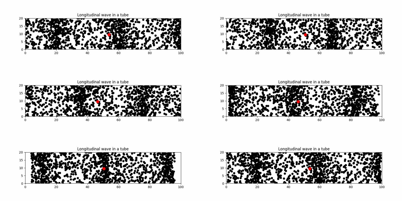
In Figure 3.1, air molecules are drawn as randomly placed particles in a tube, and one particle is tracked in red as the wave passes.
Longitudinal waves
Sound is a longitudinal wave: Figure 3.1 shows the molecules oscillating back and forth along the same direction the pattern travels, in line with the tube. In a transverse wave, by contrast, the medium oscillates perpendicular to the direction of travel, as a rope does when a displacement runs along its length. Ripples on water and the electromagnetic waves used in pulse oximetry are transverse, whereas sound in air, water, and tissue is longitudinal. The distinction becomes relevant later; within this section the two types behave identically, since both are described by the same four quantities and the same governing equation. A longitudinal wave may therefore be represented as though it were transverse, by plotting each molecule’s displacement as a vertical height, with no loss of information: exactly the convention the wave diagrams throughout this book use.
Before extending the discussion of pressure waves, it is useful to establish the general properties that describe any wave, one at a time.
Wavelength
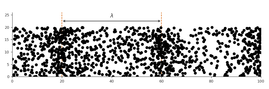
Considered at a fixed instant, the wave repeats in space: compression, rarefaction, compression, in a regular pattern. The distance between two successive pressure maxima, the peak of one compression to the peak of the next, is the wavelength \(\lambda\) (the Greek letter lambda), measured in meters. Figure 3.2 marks this distance on a single frozen instant of the tube in Figure 3.1.
Period
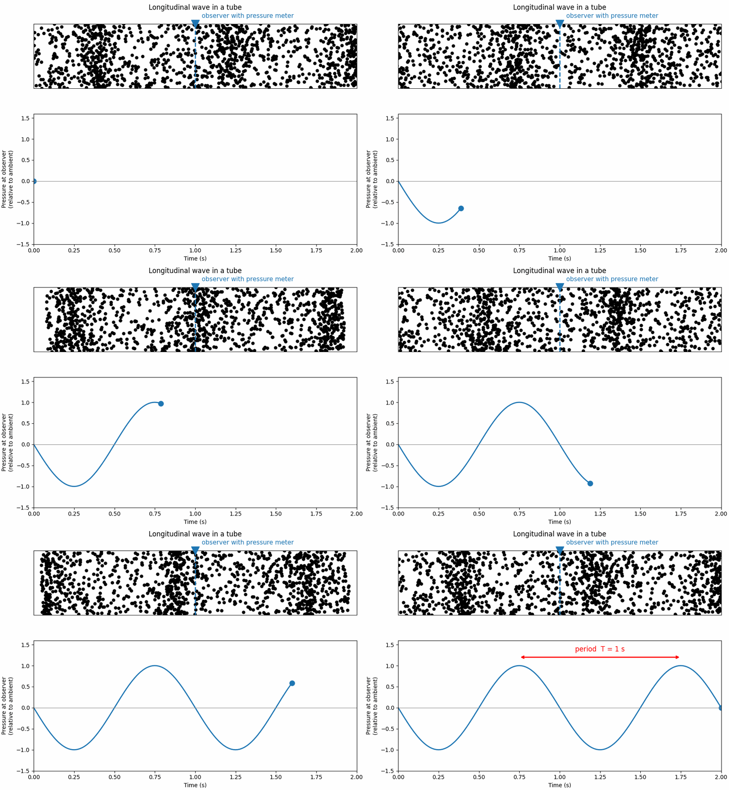
At a fixed point in space, by contrast, the air pressure rises and falls periodically as the wave passes: high, low, and back to high, repeating without end. This is the time view of the wave: how fast the pressure changes at one point, rather than how it varies across space at one instant. The time for one complete cycle is the period \(T\), measured in seconds. Wavelength is the spatial analogue of the period: the period is the repeat interval in time, and the wavelength is the repeat interval in space.
Figure 3.3 shows the period directly: a stationary observer holds a pressure meter at one point in the tube of Figure 3.1, and the trace below records what that meter reads over time. Each time a compression band sweeps past the meter, the pressure peaks; the time between successive peaks is the period \(T\).
Two views of the same wave
Wavelength and period describe the same wave from two different vantage points: wavelength is what a snapshot in space shows, period is what a fixed observer’s clock shows. A wave is therefore completely specified by four quantities. Two describe the oscillation in time at a single fixed point in space; two describe the spatial pattern at a single fixed instant. Figure 3.4 presents both descriptions of one wave side by side. Distinguishing the temporal view from the spatial view removes a common source of confusion.
import numpy as np
import matplotlib.pyplot as plt
plt.style.use("../../theme/bioe10.mplstyle")

f, v, A = 1000.0, 343.0, 1.0        # a 1 kHz tone in air
T, lam = 1 / f, v / f               # T = 1 ms, lambda = 34.3 cm

t = np.linspace(0, 2.5 * T, 500)    # left panel: displacement vs. time
x = np.linspace(0, 2.5 * lam, 500)  # right panel: displacement vs. space
# ... plot A*sin(2*pi*f*t) against t, and A*sin(2*pi*x/lam) against x,
# marking A and T on the left panel and lambda on the right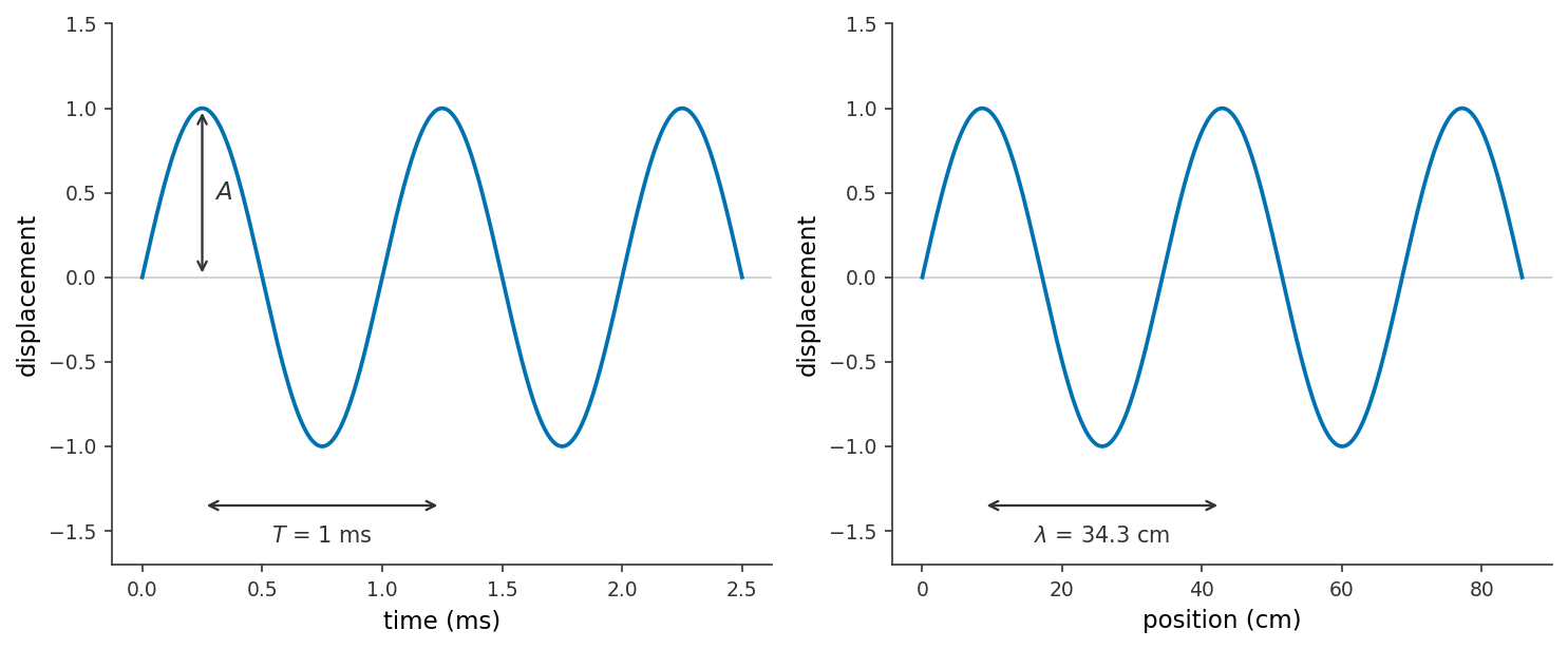
The amplitude \(A\) is the maximum displacement of the oscillation from its resting value, corresponding here to the loudness of the sound, or to the height of the peaks in the left panel of Figure 3.4.
Frequency
The reciprocal of the period is generally the more convenient quantity. The frequency \(f\) is the number of complete cycles per unit time:
\[f = \frac{1}{T}.\]
Its unit is the hertz (Hz), defined as one cycle per second, \(1~\text{Hz} = 1~\text{s}^{-1}\) (Ling et al. 2016). A wave of period \(T = 2~\text{ms}\) completes \(f = 1/0.002 = 500\) cycles per second, so \(f = 500~\text{Hz}\). For sound in the audible range this frequency determines the perceived pitch: a higher frequency corresponds to a higher pitch. Period and frequency are equivalent descriptions, expressed respectively in seconds per cycle and cycles per second, with \(f = 1/T\) converting between them.
The wave relation: \(v = f\lambda\)
The wave is characterized by a temporal repeat (\(T\), equivalently \(f\)) and a spatial repeat (\(\lambda\)). Because the pattern is in motion, these quantities are not independent: the speed at which the pattern travels must relate its spatial repeat to its temporal repeat. This relation is the central result of the section, and it is nearly determined by dimensional considerations alone.
A dimensional argument establishes the form of the relation directly. The product of a wavelength and a frequency has units
\[[\lambda]\cdot[f] = \text{m} \cdot \frac{1}{\text{s}} = \frac{\text{m}}{\text{s}},\]
which are the units of speed. Meters per second is the unit neither of a length nor of a rate alone, but of a velocity. A combination of quantities that reproduces the units of the target quantity is a strong indication of the correct relation, and the indication holds here: the product \(f\lambda\) is the speed at which the wave travels.
The dimensional argument is suggestive rather than conclusive; a short physical argument establishes the relation exactly. Because the relation is central to the section, its derivation is given in full below rather than deferred.
For any wave (sound, light, or ripples on water), the speed \(v\), frequency \(f\), and wavelength \(\lambda\) satisfy
\[\boxed{\; v = f\lambda \;} \qquad \left(v~\text{in m/s},\quad f~\text{in Hz},\quad \lambda~\text{in m}\right).\]
Equivalently \(v = \lambda/T\), since \(f = 1/T\). Any two of \(v\), \(f\), and \(\lambda\) determine the third.
The relation contains three quantities, and in practice one is typically fixed while the other two vary in inverse proportion. Which quantity is fixed is the subject of the next section, and it is what makes \(v = f\lambda\) an engineering tool rather than a mere identity.
Wave speed
The speed of a wave is a property of the medium through which it travels, not of the source that generates it (Ling et al. 2016). Sounds of different frequency and amplitude all propagate through air at \(343~\text{m/s}\), differing in frequency and amplitude but not in speed. When the frequency is changed within a fixed medium, the speed is unchanged and the wavelength adjusts to compensate, since the product \(f\lambda = v\) is fixed. Increasing \(f\) decreases \(\lambda\) in exact proportion. The complementary case is equally important. When a wave passes from one medium into another, for example from air into water, the source continues to fix its frequency, so \(f\) is preserved, while the speed \(v\) takes the value of the new medium and the wavelength changes to match (\(\lambda = v/f\)).
The speed is determined by two opposing properties of the medium. The first is its stiffness, the strength with which it resists deformation and restores itself. A stiffer medium returns each layer to its neighbor more rapidly and transmits the disturbance faster, so greater stiffness increases the speed. The second is its density, the mass per unit volume. A denser medium responds more slowly, because its greater mass is more difficult to accelerate, so greater density decreases the speed. For a fluid such as air, water, or blood, stiffness is quantified by the bulk modulus \(B\), the resistance to compression, and the two effects combine into a single expression for the speed of sound (Ling et al. 2016):
\[v = \sqrt{\frac{B}{\rho}},\]
with \(\rho\) the density. Stiffness appears in the numerator and density in the denominator, under a square root. The formula is seldom evaluated directly, but its form accounts for the representative values below:
| Medium | Speed of sound (m/s) |
|---|---|
| Air (at 20 °C) | 343 |
| Fresh water | 1480 |
| Soft tissue (average) | ~1540 |
| Bone / steel | ~4000 and up |
Table 3.1 follows the general ordering \(v_{\text{solid}} > v_{\text{liquid}} > v_{\text{gas}}\) (Ling et al. 2016). This ordering may appear paradoxical, since solids are the densest media listed and density reduces the speed. The resolution is that stiffness increases far more rapidly than density across these media: a solid is hundreds of thousands of times stiffer than a gas but only a few thousand times denser, so the stiffness term dominates under the square root. The third row is the most important for the present purpose: sound travels through soft tissue at approximately \(1540~\text{m/s}\), close to its speed in water because tissue is predominantly water, and this value is taken as the fixed speed \(c\) in \(v = f\lambda\) throughout the next section (Aldrich 2007).
- Sound is a longitudinal pressure wave (compressions and rarefactions along the direction of travel).
- Four quantities specify a wave: the period \(T\) (repeat time), the frequency \(f = 1/T\) in hertz (cycles per second), the wavelength \(\lambda\) (repeat distance), and the amplitude \(A\) (the magnitude of the oscillation).
- They are related by the wave equation \(\boxed{v = f\lambda}\) (equivalently \(v = \lambda/T\)), valid for every wave.
- The speed \(v\) is set by the medium, not the source: \(v = \sqrt{B/\rho}\) for sound in a fluid, giving \(\approx 1540~\text{m/s}\) in soft tissue.
With this vocabulary established, the next section puts it to work: choosing a frequency for medical imaging, and building an instrument around reflection, echoes, and the Doppler shift.