The scenarios are constructed for practice. Their numbers are illustrative unless a source is named.
The code defines the area tools used in sampling, categorical inference, and numerical inference: the standard normal CDF \(\Phi\), from the error function, and the \(t\)-distribution density, from the gamma function. It uses no statistics package.
import numpy as npimport matplotlib.pyplot as pltfrom math import erf, sqrt, gamma, piBLUE, GOLD, GREEN ="#0072B2", "#E69F00", "#009E73"# --- The area tools from the sampling and hypothesis-testing sections, rebuilt# here so the practice set is self-contained (no statistics package needed). ---def Phi(z):"Standard normal CDF, Phi(z) = P(Z <= z), from the error function."return0.5* (1.0+ erf(z / sqrt(2.0)))def normal_p(z):"Two-sided normal p-value: the standard-normal area beyond |z| in both tails."return2.0* (1.0- Phi(abs(z)))def normal_ppf(p):"Inverse of Phi: the z whose left-tail area is p, found by bisection." lo, hi =-8.0, 8.0for _ inrange(200): mid =0.5* (lo + hi) lo, hi = (mid, hi) if Phi(mid) < p else (lo, mid)return0.5* (lo + hi)def t_pdf(x, nu):"Student's t density with nu degrees of freedom, from the gamma function." coef = gamma((nu +1) /2) / (np.sqrt(nu * pi) * gamma(nu /2))return coef * (1+ x**2/ nu) ** (-(nu +1) /2)def t_two_sided_p(t_obs, nu):"Two-sided t p-value: twice the upper-tail area beyond |t|, by integration." xs = np.linspace(abs(t_obs), abs(t_obs) +60, 400_000)return2* np.trapezoid(t_pdf(xs, nu), xs)
Exercises
TipProblem 1
A clinic records the time to complete wound closure, in days, for nine patients treated with a skin-substitute graft:
\[ 28,\ 31,\ 34,\ 35,\ 37,\ 40,\ 44,\ 52,\ 95. \]
Compute the sample mean and the median.
The mean and median differ. Which is larger, and what does the comparison say about the shape of the distribution? Which of the two is the more representative summary of a typical patient, and why?
Compute the sample variance and sample standard deviation (dividing by \(n-1\)).
Is a histogram or a bar chart the appropriate display for these data? Give the reason in one sentence.
NoteAnswer 1
The nine values sum to \(396\), so the sample mean is \(\bar x = 396/9 = 44.0\) days. Sorted, the middle (fifth of nine) value is the median, \(37\) days.
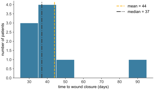
The mean (\(44.0\)) exceeds the median (\(37\)), which marks a right-skewed distribution (see Figure 31.1). The patient who took \(95\) days, far above the rest, pulls the mean upward. The median counts positions rather than magnitudes, so it stays near the bulk of the data. The median is the more representative summary of a typical patient, because it is robust to that one outlier.
Squaring each deviation from \(44.0\), summing, and dividing by \(n-1 = 8\) gives a sample variance of \(s^2 = 417.0\ \text{days}^2\) and sample standard deviation \(s = 20.4\) days (computed below). The \(n-1\) divisor is used because these nine patients are a sample, not the whole population.
A histogram. Healing time is a numerical (continuous) variable: its values lie on a number line and are grouped into bins. A bar chart is for a categorical variable, whose bars are separate labels with no numerical spacing between them.
mean   = 44.0 days
median = 37.0 days
sample variance (n-1) = 417.0 days^2
sample SD       (n-1) = 20.4 days
Figure 31.1: The nine wound-closure times, with the mean and median marked. Generated by scripts/03_statistics/10_practice/gen_practice.py.
TipProblem 2
A meal-delivery service advertises a mean delivery time of \(15\) minutes. A skeptical customer records four deliveries: \(14,\ 25,\ 15,\ 20\) minutes. Treating these as a random sample from the service’s delivery-time distribution, test at \(\alpha = 0.05\) whether the data are consistent with the advertised \(15\)-minute mean.
State \(H_0\) and \(H_1\) for a two-sided test.
Compute the sample mean, the sample standard deviation, the standard error, and the \(t\)-statistic.
Give the degrees of freedom and the two-sided p-value, and state the conclusion. Why is a \(t\)-test, rather than a z-test, the right tool here?
The observed mean came out above \(15\). Would it be legitimate to switch to a one-sided test (\(H_1:\mu > 15\)) to strengthen the case against the service? Explain.
The mean is \(\bar x = (14+25+15+20)/4 = 74/4 = 18.5\) minutes. The deviations from \(18.5\) are \(-4.5,\ 6.5,\ -3.5,\ 1.5\); their squares sum to \(77\), so the sample variance is \(s^2 = 77/(4-1) = 25.7\ \text{min}^2\) and \(s = 5.07\) minutes. The standard error is \(\mathrm{SE} = s/\sqrt n = 5.07/2 = 2.53\) minutes, and the one-sample \(t\)-statistic is \(t = (\bar x - \mu_0)/\mathrm{SE} = (18.5 - 15)/2.53 = 1.38\).
With \(\nu = n-1 = 3\) degrees of freedom, the two-sided p-value is \(\approx 0.26\) (computed below). Since \(0.26 > 0.05\), fail to reject\(H_0\): four deliveries are consistent with a \(15\)-minute mean. A \(t\)-test is the right tool because the population standard deviation is unknown (it is estimated by \(s\)) and the sample is small (\(n=4\)), so the standardized statistic follows the heavier-tailed \(t\)-distribution, not the normal.
No. The direction of a one-sided test must be fixed before the data are seen, on the grounds that a difference the other way would be of no interest. Switching to \(H_1:\mu>15\)after seeing the sample mean land above \(15\) would halve the p-value, but it inflates the true Type I error rate above the stated \(0.05\) and is not a valid test.
delivery = np.array([14, 25, 15, 20]) # minutes, 4 deliveriesn = delivery.sizexbar = delivery.mean()s = delivery.std(ddof=1)se = s / np.sqrt(n)t = (xbar -15) / sep = t_two_sided_p(t, nu=n -1)print(f"mean = {xbar:.1f} min, s = {s:.2f} min, SE = {se:.2f} min")print(f"t = {t:.2f} on nu = {n-1} degrees of freedom")print(f"two-sided p-value = {p:.3f} -> {'reject'if p <=0.05else'fail to reject'} H0 at alpha = 0.05")
mean = 18.5 min,  s = 5.07 min,  SE = 2.53 min
t = 1.38  on nu = 3 degrees of freedom
two-sided p-value = 0.261  ->  fail to reject H0 at alpha = 0.05
TipProblem 3
Suppose SAT scores on some administration are approximately normal with mean \(1500\) and standard deviation \(300\) (illustrative figures, on the traditional \(2400\)-point scale), and ACT scores are approximately normal with mean \(21\) and standard deviation \(5\). One applicant scored \(1800\) on the SAT; another scored \(24\) on the ACT. The two scales are not directly comparable.
Standardize each score to a z-score.
Which applicant scored better relative to the population taking their test?
Using the standard normal, what percentile does each z-score correspond to (the fraction scoring below)? Relate the SAT applicant’s percentile to the 68–95–99.7 rule.
NoteAnswer 3
The z-score \(z = (x-\mu)/\sigma\) rescales each score to the standard normal. \(z_{\text{SAT}} = (1800-1500)/300 = 1.0\) and \(z_{\text{ACT}} = (24-21)/5 = 0.6\).
The SAT applicant. A z-score of \(1.0\) stands one standard deviation above its mean, against \(0.6\) for the ACT applicant. Because the raw scales differ, each score is compared with its own population, and the SAT applicant ranks higher.
The percentile is the standard-normal area below the z-score, \(\Phi(z) = P(Z \leq z)\): \(\Phi(1.0) \approx 0.841\) and \(\Phi(0.6) \approx 0.726\), so the SAT applicant is at about the 84th percentile and the ACT applicant at about the 73rd (computed below). The 68–95–99.7 rule reproduces the first without a table: \(68\%\) of a normal distribution lies within \(\pm 1\) SD, leaving \(32\%\) outside, of which half (\(16\%\)) lies above \(+1\) SD. So \(84\%\) lies below it, which matches \(\Phi(1) \approx 0.841\) to rounding.
A z-score is a standardization, not a hypothesis test: there is no null hypothesis and no p-value here, only the location of a value within its distribution.
SAT applicant: z = 1.00  ->  84.1th percentile
ACT applicant: z = 0.60  ->  72.6th percentile
better relative to peers: SAT applicant
TipProblem 4
Healthy human body temperature is approximately normal with mean \(98.2\,°\text{F}\) and standard deviation \(0.73\,°\text{F}\)(Mackowiak et al. 1992). A clinic wishes to flag unusually low temperatures.
Using the 68–95–99.7 rule, give the temperature range that contains the central \(95\%\) of healthy people, and state what fraction fall below its lower edge.
Find the exact cutoff below which the lowest \(3\%\) of healthy body temperatures lie. Use the inverse of the standard normal to get the z-score, then convert to \(°\text{F}\).
Compare the part-(b) cutoff with the lower edge from part (a). Is it above or below that edge, and why is that the direction to expect?
NoteAnswer 4
For a normal variable the central \(95\%\) lies within \(\pm 2\) standard deviations of the mean: \(98.2 \pm 2(0.73) = 98.2 \pm 1.46 = [96.74\,°\text{F},\ 99.66\,°\text{F}]\). The rule leaves \(5\%\) outside, split between the two tails, so about \(2.5\%\) fall below the lower edge of \(96.74\,°\text{F}\).
The lowest \(3\%\) lie below the z-score with \(\Phi(z) = 0.03\), which is \(z \approx -1.88\) (the inverse of the standard normal CDF). Converting back to temperature with \(x = \mu + z\sigma\): \(x = 98.2 + (-1.88)(0.73) \approx 96.83\,°\text{F}\) (computed below).
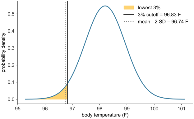
The \(3\%\) cutoff (\(96.83\,°\text{F}\)) lies above the \(2.5\%\) edge (\(96.74\,°\text{F}\)) (see Figure 31.2). This is the expected direction: a larger tail fraction (\(3\% > 2.5\%\)) reaches less far into the low tail, so its cutoff sits closer to the mean, at a higher temperature. The two agree to within about a tenth of a degree; the exact inverse-normal calculation refines the \(\pm 2\)-SD estimate from the rule.
central 95% range: [96.74, 99.66] F
z for lowest 3% = -1.88  ->  cutoff = 96.83 F
2.5% edge (mean - 2 SD) = 96.74 F   (3% cutoff sits just above it)
Figure 31.2: The body-temperature distribution, with the lowest-3% cutoff and the mean-minus-2SD edge marked. Generated by scripts/03_statistics/10_practice/gen_practice.py.
A historical control is a comparison figure taken from earlier records, and a concurrent control is a control group treated at the same time as the treated group. A systematic error (bias) pushes every measurement or comparison in the same direction. Unlike the random variation that shrinks as \(n\) grows, a systematic error does not shrink.
TipProblem 5
Under standard care, recovery after a severe burn takes a mean of \(215\) days. A manufacturer claims its skin-substitute graft speeds recovery. An independent group applies the graft to a random sample of \(n = 30\) burn patients. The sample mean recovery time is \(\bar x = 204\) days, and the sample standard deviation is \(s = 25\) days. The population standard deviation is unknown, so use a t-test.
The group decided in advance to test whether the graft reduces recovery time. State \(H_0\) and \(H_1\) accordingly (a one-sided test). Give the degrees of freedom, and the distribution of \(t = (\bar x - \mu_0)/(s/\sqrt n)\) under \(H_0\).
Compute the standard error of the sample mean and the t-statistic.
Give the one-sided p-value and the conclusion at \(\alpha = 0.05\). Report the two-sided p-value as well.
This study compares the treated sample against a fixed historical mean rather than against a concurrent control arm. Name one systematic error (bias) that the design leaves open, a difference that does not shrink as \(n\) grows. The two-arm Dermagraft trial guarded against it. State its consequence for the result.
NoteAnswer 5
\(H_0: \mu = 215\) days (the graft does not reduce recovery); \(H_1: \mu < 215\) days (it reduces it). Under \(H_0\), the statistic \(t = (\bar x - 215)/(s/\sqrt n)\) follows a \(t\)-distribution with \(\nu = n - 1 = 29\) degrees of freedom.
\(\mathrm{SE} = s/\sqrt n = 25/\sqrt{30} = 4.56\) days. The t-statistic is \(t = (\bar x - \mu_0)/\mathrm{SE} = (204 - 215)/4.56 = -2.41\).
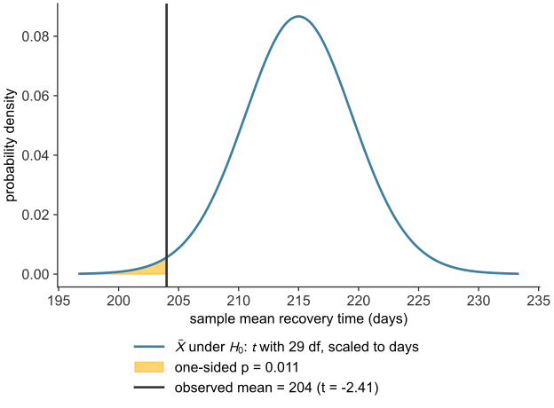
The one-sided (lower-tail) p-value is the area of the \(t_{29}\) distribution below \(-2.41\), which is \(p \approx 0.011\) (see Figure 31.3). Since \(0.011 \leq 0.05\), reject\(H_0\): the sample gives significant evidence that the graft reduces recovery time. The two-sided p-value is \(0.023\), also below \(0.05\), so the conclusion does not hinge on the one-sided choice.
The design has no concurrent control: the \(11\)-day improvement is measured against a historical figure, not against a group treated alongside the sample. Any difference between the sample and the era or population behind the \(215\)-day standard, such as improved routine care, a healthier patient mix, or milder injuries, is a confounder that could produce the difference even if the graft had no effect. Such a systematic error (bias) does not shrink with sample size, and a significance test cannot detect it. The two-arm Dermagraft trial guarded against this by running its control arm concurrently, under identical conditions.
mu0, n5, xbar5, s5 =215, 30, 204, 25# historical mean; sample size, mean, SDse5 = s5 / np.sqrt(n5)t5 = (xbar5 - mu0) / se5p_one = t_two_sided_p(t5, nu=n5 -1) /2# lower-tail area (H1: mu < mu0)p_two =2* p_oneprint(f"SE = s/sqrt(n) = {se5:.2f} days")print(f"t = {t5:.2f} on nu = {n5 -1} degrees of freedom")print(f"one-sided p = {p_one:.4f} two-sided p = {p_two:.4f}")print(f"conclusion: {'reject'if p_one <=0.05else'fail to reject'} H0 (one-sided, alpha = 0.05)")
SE = s/sqrt(n) = 4.56 days
t = -2.41  on nu = 29 degrees of freedom
one-sided p = 0.0113   two-sided p = 0.0225
conclusion: reject H0 (one-sided, alpha = 0.05)
Figure 31.3: The sampling distribution of the mean under \(H_0\), drawn as a \(t\)-distribution with 29 degrees of freedom and scaled to days, with the observed mean and the one-sided p-value shaded. Generated by scripts/03_statistics/10_practice/gen_practice.py.
TipProblem 6
A trial tests whether a new drug lowers systolic blood pressure more than a placebo. The outcome is the reduction in systolic pressure (mmHg) over the treatment period. A larger reduction is better. Seven patients per arm give:
Drug:\(10,\ 12,\ 13,\ 15,\ 17,\ 19,\ 20\)
Placebo:\(8,\ 9,\ 11,\ 11,\ 12,\ 13,\ 15\)
Test at \(\alpha = 0.05\), two-sided, whether the mean reductions differ. Do not assume the two arms have equal spread. Use the two-sample t-test with the conservative degrees of freedom, the smaller of \(n_1 - 1\) and \(n_2 - 1\).
State \(H_0\) and \(H_1\).
Compute each group’s mean and sample standard deviation, and the standard error of the difference.
Compute the \(t\)-statistic and its degrees of freedom, give the two-sided p-value, and state the conclusion.
\(t = (\bar x_1 - \bar x_2)/\mathrm{SE} = (15.14 - 11.29)/1.66 = 2.32\). The degrees of freedom are the smaller of \(n_1 - 1 = 6\) and \(n_2 - 1 = 6\), so \(\nu = 6\). The two-sided p-value is \(\approx 0.060\) (computed below). Since \(0.060 > 0.05\), fail to reject\(H_0\): the data do not show a significant difference in mean reduction, although the drug arm’s mean is \(3.9\) mmHg higher.
Note: Software uses Welch’s approximate degrees of freedom instead, \(\nu = \dfrac{(s_1^2/n_1 + s_2^2/n_2)^2}{(s_1^2/n_1)^2/(n_1 - 1) + (s_2^2/n_2)^2/(n_2 - 1)} \approx 10.2\). That gives \(p \approx 0.043\), which would reject \(H_0\). Welch’s rule uses both groups’ variances. The conservative rule uses only the smaller group’s size, so it overstates the uncertainty when the groups differ in spread. Here the result sits close to the \(0.05\) boundary, so the choice matters.
drug = np.array([10, 12, 13, 15, 17, 19, 20]) # mmHg reduction, 7 patientsplacebo = np.array([8, 9, 11, 11, 12, 13, 15])n1, n2 = drug.size, placebo.sizes1, s2 = drug.std(ddof=1), placebo.std(ddof=1)se = np.sqrt(s1**2/ n1 + s2**2/ n2) # SE of the differencet = (drug.mean() - placebo.mean()) / sedof =min(n1 -1, n2 -1) # conservative degrees of freedomp = t_two_sided_p(t, nu=dof)print(f"drug: mean = {drug.mean():.2f} mmHg, s = {s1:.2f}")print(f"placebo: mean = {placebo.mean():.2f} mmHg, s = {s2:.2f}")print(f"SE of difference = {se:.2f}")print(f"t = {t:.2f} on nu = {dof} degrees of freedom")print(f"two-sided p = {p:.3f} -> {'reject'if p <=0.05else'fail to reject'} H0")
drug:    mean = 15.14 mmHg,  s = 3.72
placebo: mean = 11.29 mmHg,  s = 2.36
SE of difference = 1.66
t = 2.32  on nu = 6 degrees of freedom
two-sided p = 0.060  ->  fail to reject H0
TipProblem 7
A clinical trial tests a new drug against a placebo, with a binary endpoint: whether each patient showed clinically meaningful improvement. Of \(160\) patients on the drug, \(96\) improved; of \(160\) on the placebo, \(72\) improved. Test at \(\alpha = 0.05\), two-sided, whether the drug changes the improvement rate.
State \(H_0\) and \(H_1\) in terms of the two population rates. Give the two observed rates and their difference.
Test \(H_0\) with the pooled standard error. Compute the pooled rate, the standard error of the difference, the z-statistic, and the two-sided p-value. State the conclusion. Why is a z-test used rather than a t-test for this outcome?
Construct a \(95\%\) confidence interval for \(p_1 - p_2\), using the unpooled standard error of the difference. Does the interval agree with the test in (b)?
NoteAnswer 7
\(H_0: p_1 = p_2\) (the drug does not change the improvement rate); \(H_1: p_1 \neq p_2\). The observed rates are \(\hat p_1 = 96/160 = 0.600\) and \(\hat p_2 = 72/160 = 0.450\), a difference of \(0.150\) (\(15\) percentage points).
Under \(H_0\) the two rates are equal, so both arms share one pooled rate, \(\hat p = 168/320 = 0.525\). The standard error of the difference is \(\mathrm{SE}_{\text{pool}} = \sqrt{\hat p(1-\hat p)(1/160 + 1/160)} = 0.0558\). Then \(z = 0.150/0.0558 = 2.69\), and the two-sided p-value is \(2\big(1-\Phi(2.69)\big) \approx 0.007\), where \(\Phi(z)\) is the standard normal area to the left of \(z\). Since \(0.007 \leq 0.05\), reject\(H_0\): the improvement rates differ significantly. A z-test is used because the variance of a proportion is fixed by the rate, \(p(1-p)\), so no separate spread needs estimating. Each arm has \(160\) patients, so the normal approximation holds.
The unpooled standard error is \(\sqrt{\hat p_1(1-\hat p_1)/160 + \hat p_2(1-\hat p_2)/160} = 0.0552\). The interval is \(0.150 \pm 1.96 \times 0.0552 = 0.150 \pm 0.108\), or \((0.042,\ 0.258)\). In percentage points, the drug’s effect lies between \(4.2\) and \(25.8\) points. The interval excludes \(0\), which agrees with rejecting \(H_0\) in (b).
rates: p1 = 0.600, p2 = 0.450, difference = 0.150
pooled: p_hat = 0.525  SE = 0.0558  z = 2.69  two-sided p = 0.007
unpooled: SE = 0.0552   95% CI = (0.042, 0.258)
TipProblem 8
A company reports the following study of a new wound-healing device.
We treated\(80\) patients at our clinic with the device. Physicians selected the patients they judged most likely to benefit. At twelve weeks, \(60\%\) had healed — far above the \(35\%\) healing rate in a different hospital’s records from five years earlier. The treating physicians, who knew each patient had received the device, assessed healing by visual inspection. We conclude the device works.
The reported difference is large and would be highly statistically significant. The design, however, is unsound. Identify the systematic errors, and for each name the design feature that would remove it.
Is there a valid control group? What comparison was used instead, and why is it untrustworthy?
How were patients assigned to treatment, and what bias does that invite?
Who assessed the outcome, and what bias does that invite?
In one sentence, explain why the large, “highly significant” difference does not establish that the device works.
NoteAnswer 8
(a) No concurrent control. The \(60\%\) is compared against a historical figure: another hospital’s records from five years earlier. Standards of care, patient mix, and how “healed” is judged all drift across time and centers, so any of those differences could produce the \(60\%\)-versus-\(35\%\) difference instead of the device. The fix is a concurrent control arm, a control group treated at the same time as the device group, drawn from the same population, managed identically except for the device.
(b) Assignment by physician judgment. Physicians selected the patients “most likely to benefit,” which makes patient prognosis a confounding variable: the treated group is stacked with easy cases and could heal more often even if the device did nothing. The fix is randomization: it makes arm membership independent of prognosis and of other patient characteristics, measured or not.
(c) Unblinded assessment. The outcome was judged by the treating physicians, who knew each patient had received the device. An assessor who knows the assignment can read ambiguous cases in the expected direction, an assessment bias. The fix is blinding the outcome assessor: healing is judged by an evaluator who does not know which treatment each patient received (for instance, from coded photographs).
Statistical significance rules out only chance as an explanation. It says nothing about bias, and the study’s difference could be produced entirely by its uncontrolled, non-randomized, unblinded design.
Adhikari, Ani, John DeNero, and David Wagner. 2022. Computational and Inferential Thinking: The Foundations of Data Science. 2nd ed. University of California, Berkeley (Data 8). https://inferentialthinking.com/.
Mackowiak, Philip A., Steven S. Wasserman, and Myron M. Levine. 1992. “A Critical Appraisal of 98.6 Degrees F, the Upper Limit of the Normal Body Temperature, and Other Legacies of CarlReinholdAugustWunderlich.”JAMA 268 (12): 1578–80. https://doi.org/10.1001/jama.1992.03490120092034.
Marston, William A., Jason Hanft, Paul Norwood, and Richard Pollak. 2003. “The Efficacy and Safety of Dermagraft in Improving the Healing of Chronic Diabetic Foot Ulcers: Results of a Prospective Randomized Trial.”Diabetes Care 26 (6): 1701–5. https://doi.org/10.2337/diacare.26.6.1701.