11 Signals and Systems
The heart’s electrical signal is a continuous voltage varying over time. A computer, however, stores only a list of numbers. Somewhere between the electrode on the skin and the value on a computer, the continuous voltage must be turned into 0s ans 1s.
An analog-to-digital converter, or ADC, is the hardware component that sits between the voltage sensor and the computer. It takes the analog signal and turns it into a digital bitstream (Figure 11.1).
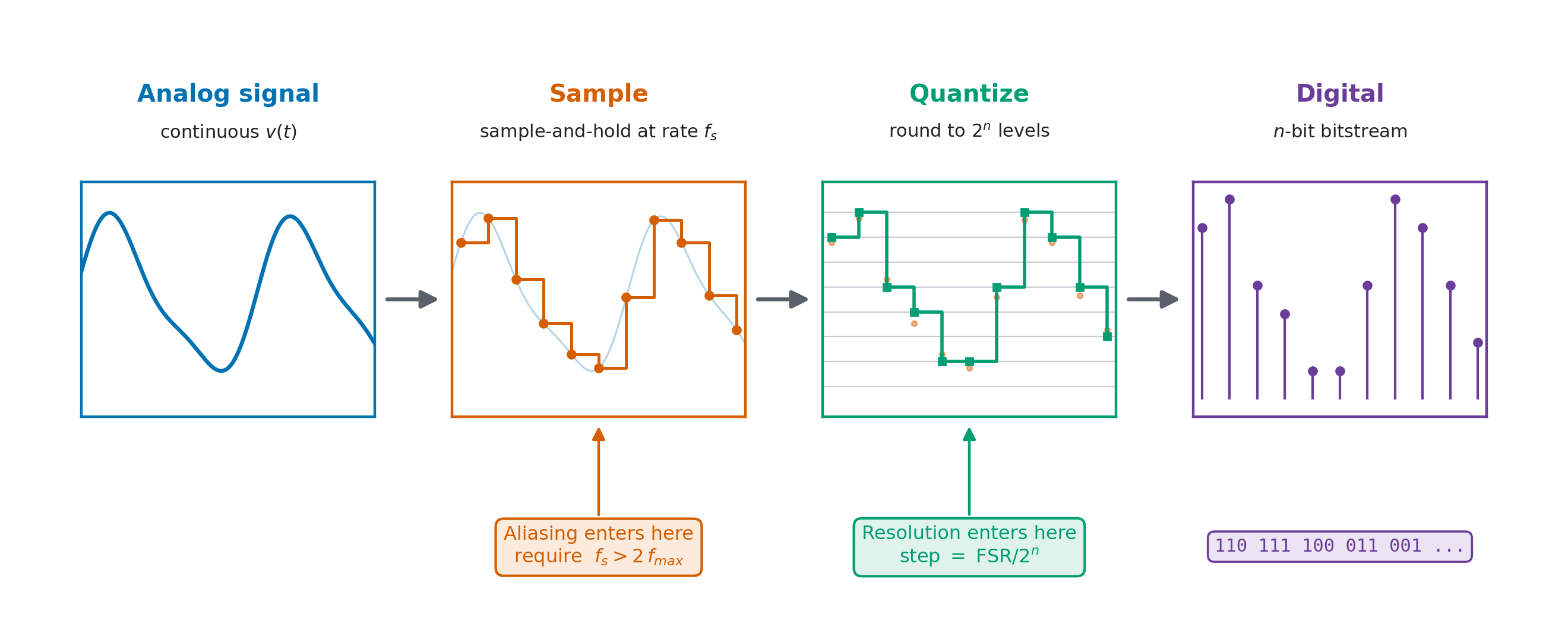
scripts/gen_signals_pipeline.py.
Continuous Signals
A continuous signal is a real number that can take on any value within a range and is defined at every time \(t\) (Figure 11.2).
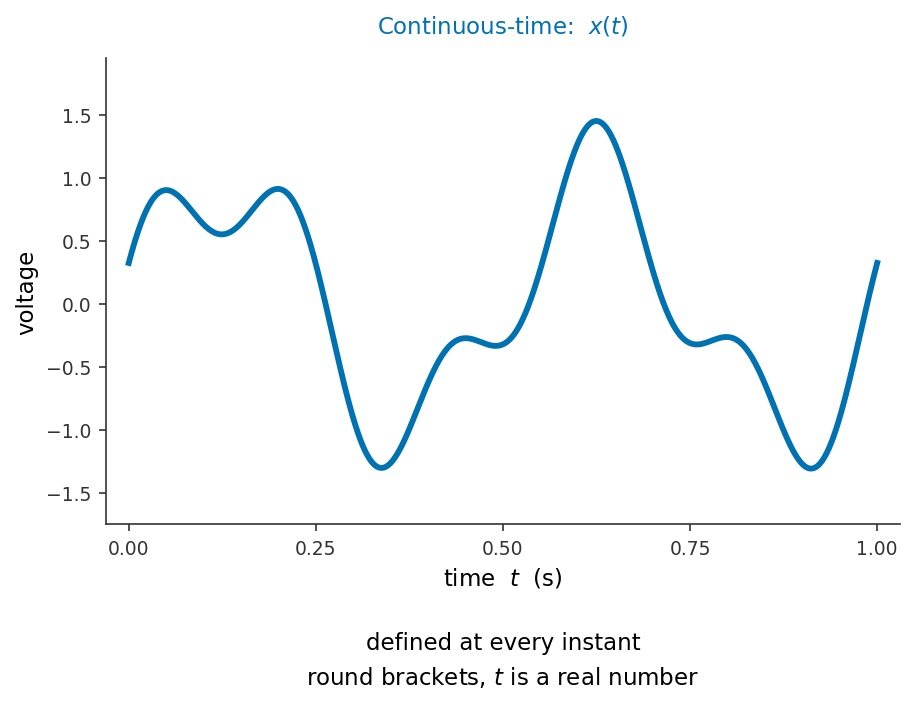
images/01_measuring/11_signals_systems/gen_l5_ct_dt.py.
Discrete Signals
A discrete signal is a sequence of numbers, each representing the signal’s value at a specific point in time. Unlike a continuous signal, it is defined only at these discrete instants, typically spaced by a fixed sampling interval \(\Delta t\) (Figure 11.3).
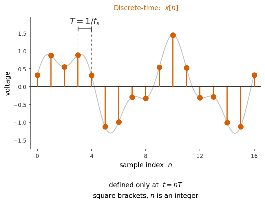
images/01_measuring/11_signals_systems/gen_l5_ct_dt.py.
To understand how to correctly sample a continuous signal, let’s review sinusoids. This is important because nearly any signal can be broken into a sum of sinusoids.
Why sinusoids?
Signals occur in unlimited variety. However any signal, however complicated, can be represented as a sum of sinusoids.
Let’s consider the signal in our earlier example. It rises to unequal peaks and has a small ripple riding on a slow swing — but it is nothing more than two sine waves added together: one of amplitude 1 at 2 Hz, and a smaller one of amplitude 0.45 at 5 Hz, shifted in phase by 0.8 rad (Figure 11.4).
import numpy as np

t = np.linspace(0, 1.0, 2000)

first  = 1.00 * np.sin(2 * np.pi * 2.0 * t)              # A = 1.00, f = 2 Hz
second = 0.45 * np.sin(2 * np.pi * 5.0 * t + 0.8)        # A = 0.45, f = 5 Hz, phi = 0.8

signal = first + second                                  # the continuous signal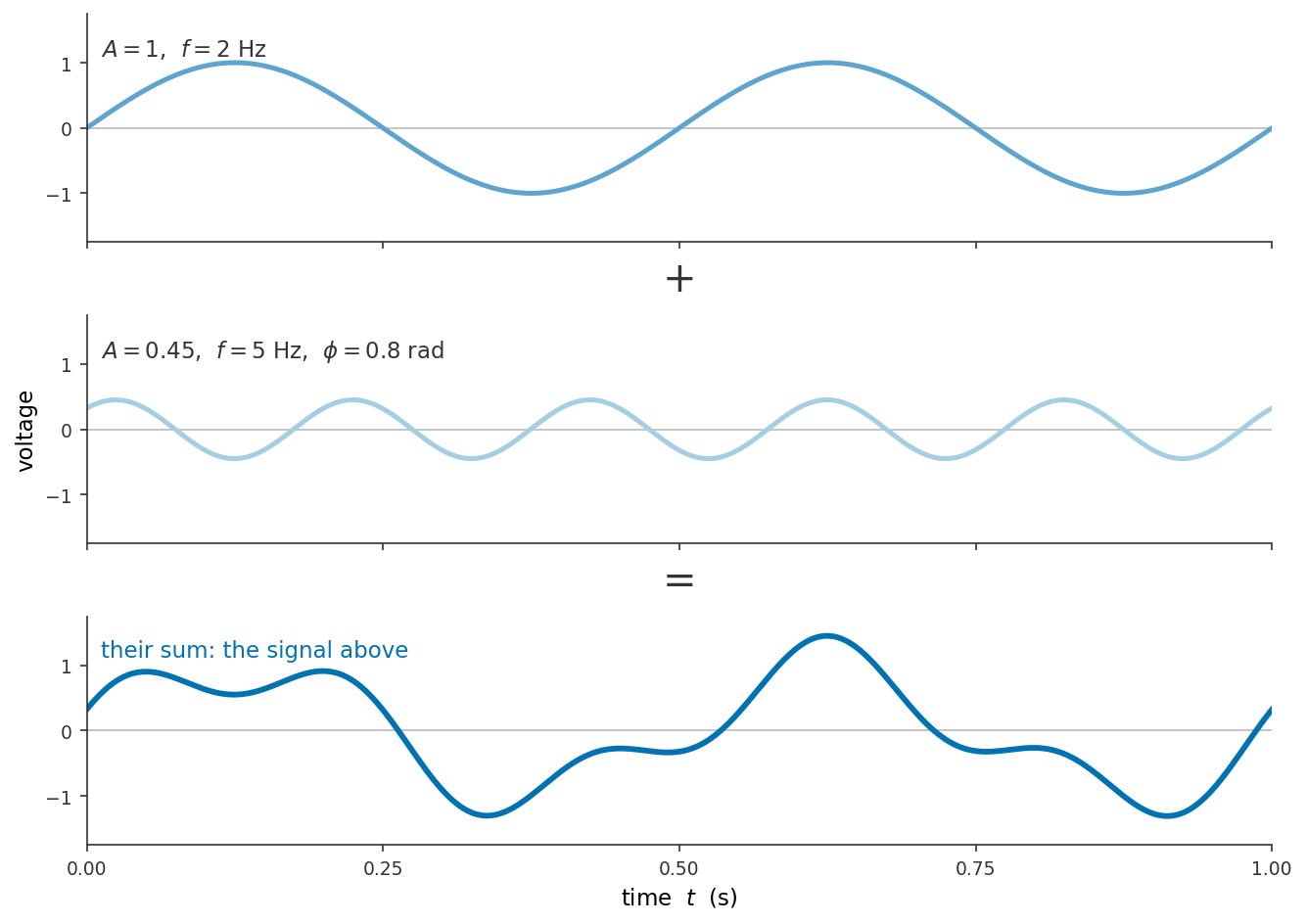
images/01_measuring/11_signals_systems/gen_l5_ct_dt.py.
Real signals are typically approximated by many sinusoids, and a square wave needs infinitely many — its sharp corners are assembled from ever-higher harmonics. However, the general principle holds: the decomposition of a signal into sines and cosines of different frequencies is possible. You will learn this, and it’s mathmatical form when you discuss Fourier analysis in other classses. It is why sinusoids are the natural building blocks of signal processing.
The Sinusoid
An angle can be measured in degrees, but for waves the natural unit is the radian. One radian is the angle subtended at the centre of a circle by an arc exactly one radius long. Measuring an angle in radians therefore amounts to counting how many radii of arc it cuts off: an angle \(\theta\) subtends an arc of length
\[s = r\,\theta .\]
Rearranged, \(\theta = s/r\) is a length divided by a length, so an angle in radians is a pure number and carries no units of its own. Go once around the circle and the arc becomes the entire circumference, \(s = 2\pi r\), so the angle of a full revolution is
\[\theta = \frac{2\pi r}{r} = 2\pi .\]
The radius cancels, which is why a full turn is \(2\pi\) radians for a circle of any size. Figure 11.5
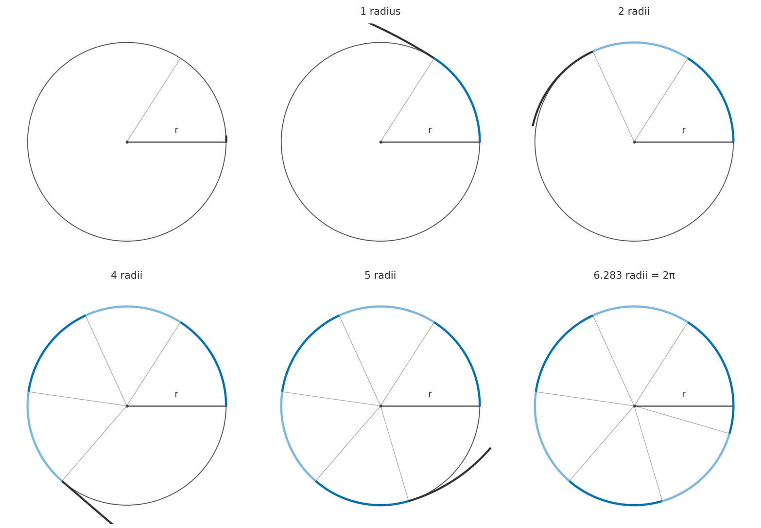
images/01_measuring/11_signals_systems/radian_demo.py.
A sine wave is the height of a point travelling around a circle (Figure 11.6). The argument of the sine is therefore an angle: one full lap is \(2\pi\) radians.
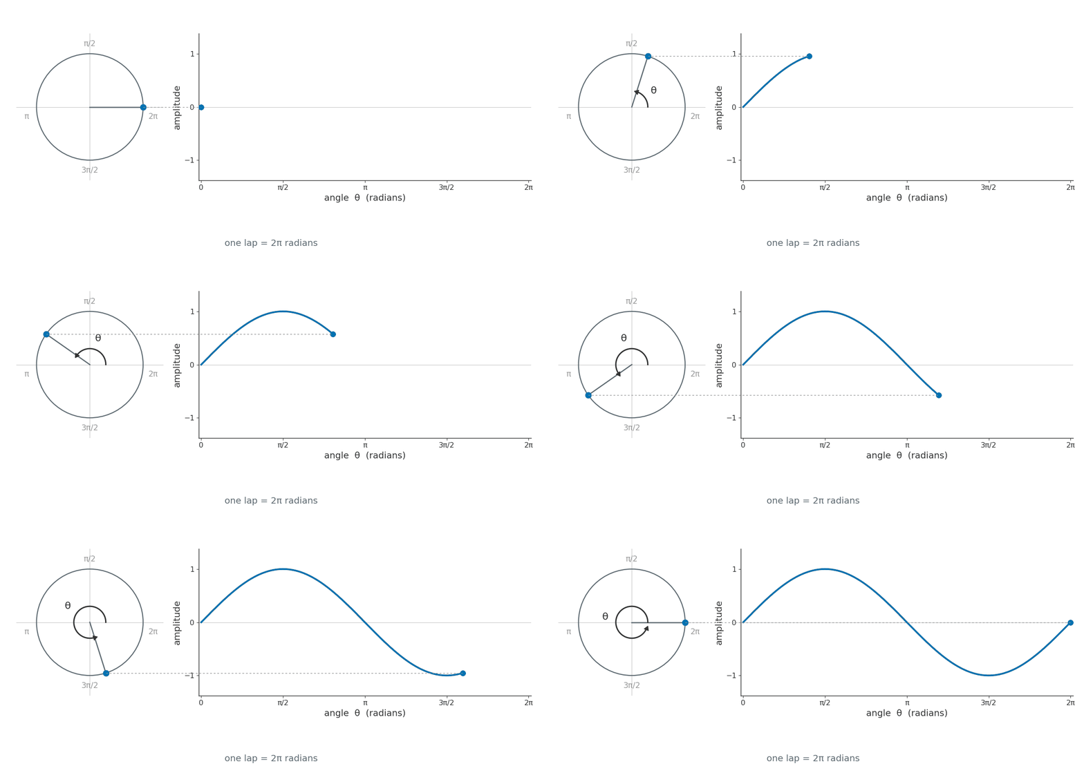
images/01_measuring/11_signals_systems/sine_nomenclature.py.
The Sinusoid V(t)
A signal as a function of time can be written as
\[v(t) = A \sin(\omega t),\]
where:
- \(A\) — the amplitude
- \(\omega\) — the angular frequency, in radians per second
The angle inside the sine advances at \(\omega\) radians per second, and one full cycle takes \(T\) seconds and covers \(2\pi\) radians, so
\[\omega = \frac{2\pi}{T}.\]
The period is the reciprocal of the frequency, \(T = 1/f\), so this can equally be written
\[\omega = 2\pi f,\]
and the wave itself becomes
\[v(t) = A \sin(2 \pi f t).\]
Finally, the wave can be shifted left or right by \(\phi\), the phase:
\[v(t) = A \sin(2 \pi f t + \phi),\]
Move the sliders to see what each of the three numbers does to the wave. Watch the period \(T = 1/f\) reported beneath the plot as you change the frequency.
Sampling Rate
The rate at which samples are taken is the sampling rate (or sampling frequency) \(f_s\), measured in samples per second, called hertz. It sets the spacing between samples, the sampling interval:
\[\Delta t = \frac{1}{f_s}.\]
At \(f_s = 500~\text{Hz}\) an EKG yields one voltage reading every \(\Delta t = 1/500 = 2~\text{ms}\), so a 10-second strip becomes a list of \(500 \times 10 = 5000\) numbers.
Let’s consider how our EKG is recorded at different sampling rates
Figure 11.7 records the same four beats at different sampling frequencies. At 500 Hz the dots are dense enough to draw the waveform on their own. Going down the panels, the samples thin out: the T wave coarsens, then the P wave becomes a couple of dots, and by 25 Hz the QRS complex survives as one or two samples.
Look at the R peaks in the bottom panel. They are recorded at 1.05, 1.01, 0.76 and 0.45 mV, a spread of 603 µV, from the same patient, in the same three seconds. Below a sufficient rate, what you measure depends on where the samples happen to land.
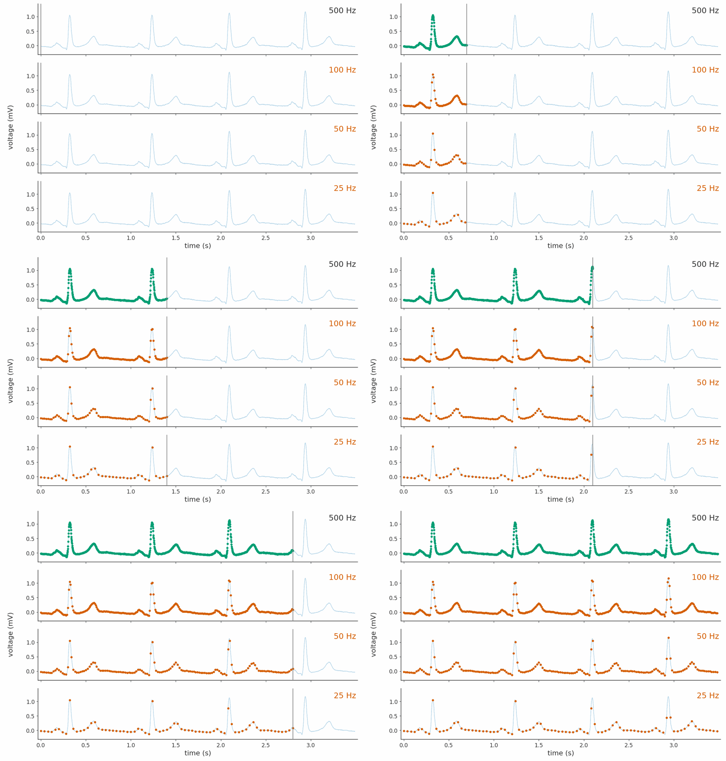
images/01_measuring/11_signals_systems/sampling_rates_panels.py.
Min sampling rate
Clearly how frequently we sample matters! But how frequent is enough? Again let’s return to the the fact that a signal can be approximated by a series of sine waves.
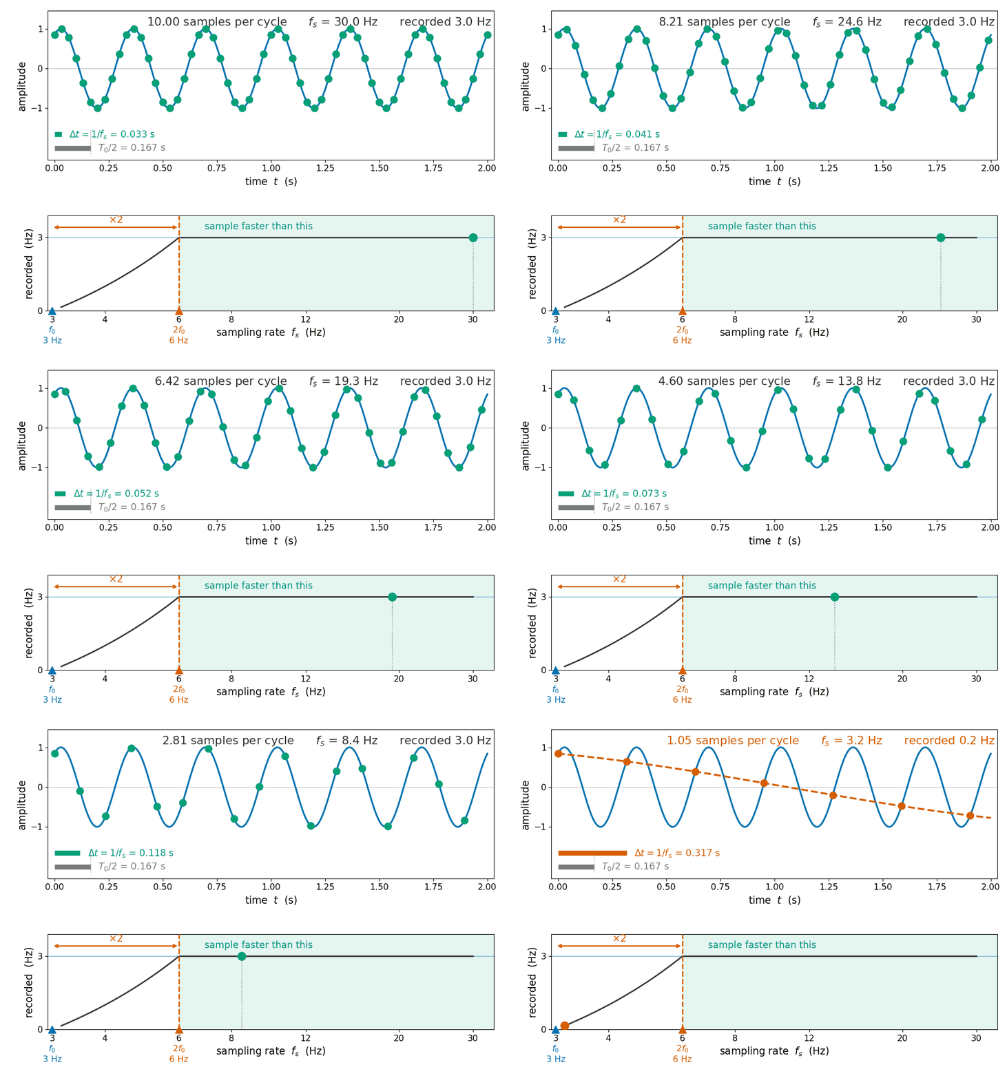
Sampling too slowly produces an effect more serious than the loss of fine detail: a high-frequency sinusoid becomes indistinguishable from a lower-frequency one. This effect is called aliasing and it is seen more clearly in Figure 11.8.
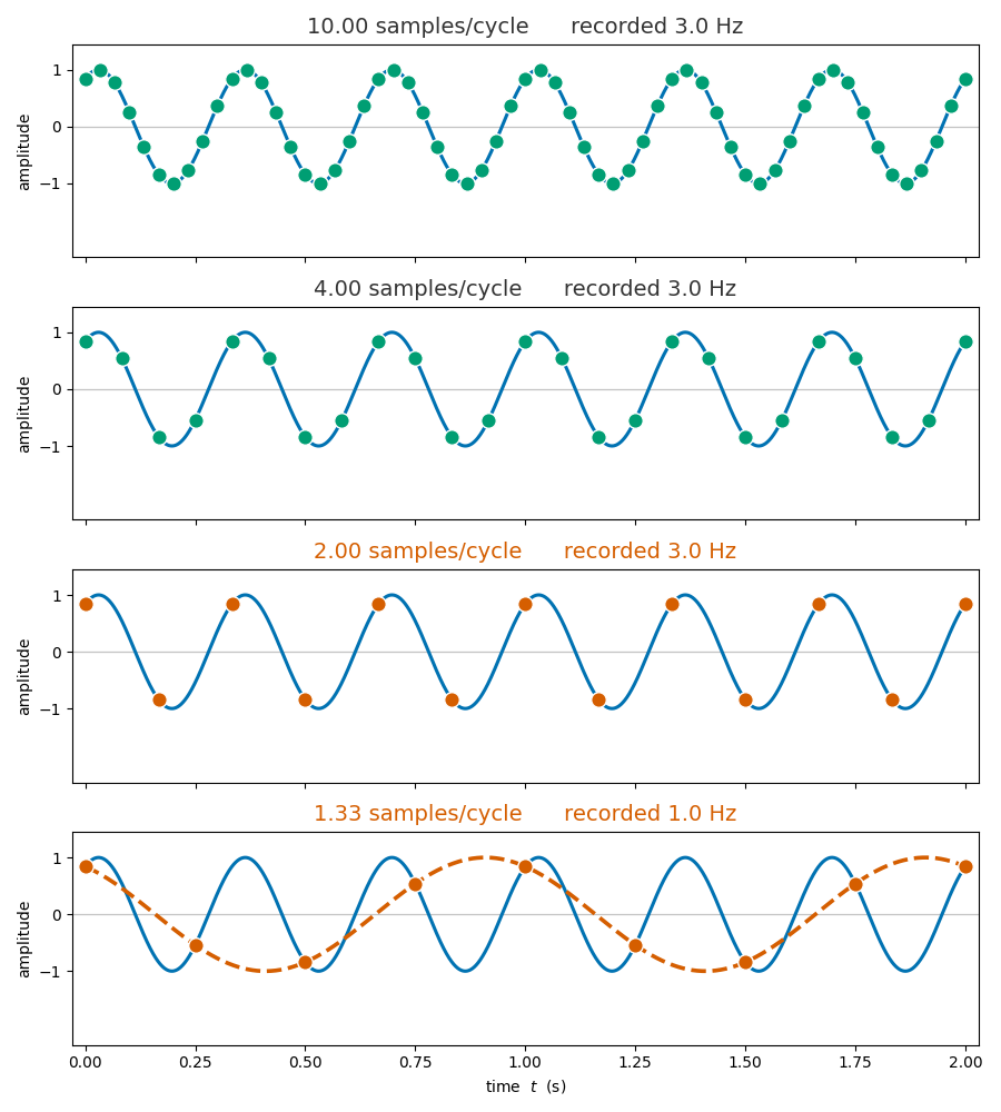
images/01_measuring/11_signals_systems/sampling_rate_sweep_hz.py.
The recorded frequency of an undersampled component is set by the signal frequency and the sampling rate together. A component of true frequency \(f_\text{signal}\) is recorded as
\[f_\text{alias} = \left| f_\text{signal} - n f_s \right|,\]
where:
- \(f_\text{signal}\) — the true frequency of the component
- \(f_s\) — the sampling rate
- \(n\) — the integer that brings the result into the range 0 to \(f_s/2\), which is the nearest integer to \(f_\text{signal}/f_s\)
The bottom panel of Figure 11.8 shows this. There the \(3~\text{Hz}\) wave is sampled at 1.33 samples per cycle, so \(f_s = 4~\text{Hz}\) and the nearest integer to \(3/4\) is \(n = 1\), giving \(f_\text{alias} = |3 - 4| = 1~\text{Hz}\). Note that the alias is a real, well-defined frequency, which is what makes undersampling so problematic.
The Nyquist–Shannon sampling theorem
Let the highest frequency present in the signal be \(f_\text{max}\). To capture this signal accurately, the sampling rate must be greater than twice this maximum frequency:
\[f_s > 2 f_\text{max}.\]
The threshold \(2 f_\text{max}\) is the Nyquist rate. Sampling below it causes aliasing, in which high-frequency components masquerade as lower-frequency ones. Sampling exactly at it is not sufficient either: two samples per cycle can land anywhere on the wave, including on every zero crossing, in which case every sample reads zero.
This is visually demonstrated in the following example.
NoteKey result: the Nyquist–Shannon sampling theorem
A signal that contains no frequency higher than \(f_{\max}\) is completely and faithfully captured by its samples if the sampling rate satisfies
\[\boxed{\; f_s > 2\,f_{\max} \;}\]
Sampling below twice the highest frequency present causes that frequency to alias into a lower one, corrupting the record irreparably; sampling at exactly twice it leaves the amplitude and phase undetermined. The threshold \(2 f_{\max}\) is the Nyquist rate, and half the sampling rate, \(f_s/2\), is the Nyquist frequency: a given ADC can represent only frequencies below it (Shannon 1949; Baraniuk and contributors 2009).
Exercises
References
Baraniuk, Richard, and contributors. 2009. Signals and Systems. OpenStax CNX / Rice University. https://eng.libretexts.org/Bookshelves/Electrical_Engineering/Signal_Processing_and_Modeling/Signals_and_Systems_(Baraniuk_et_al.)/10\%3A_Sampling_and_Reconstruction.
Shannon, Claude E. 1949. “Communication in the Presence of Noise.” Proceedings of the IRE 37 (1): 10–21. https://doi.org/10.1109/JRPROC.1949.232969.