16 Diffusion
Diffusion is the net spreading of a species down its own concentration gradient by random molecular motion, with no bulk movement of the surrounding medium. How can random motion lead to net movement of molecules? This section derives the one-dimensional mean-squared displacement \(\langle x^2\rangle = 2Dt\) from first principles using a random walk model (Phillips et al. 2012).
Building the random walk
Consider a particle at position \(x = 0\) at time \(t = 0\), on a line marked off in steps of \(\Delta x\) (Figure 16.1). At each time step \(\Delta t\) it moves either \(+\Delta x\) or \(-\Delta x\) with equal probability \(p = 1/2\). The figures that follow track where it can be after one step, two steps, and three.
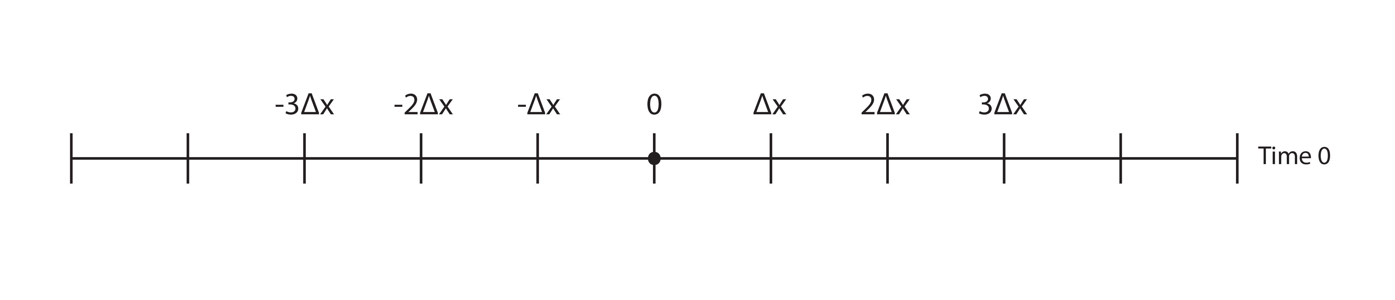
Expected displacement is zero
Because each step is symmetric, the average position is always the starting point. Angle brackets \(\langle\,\cdot\,\rangle\) denote that average: the value of a quantity weighted by how probable it is, taken over many walkers. The expected displacement after one step is:
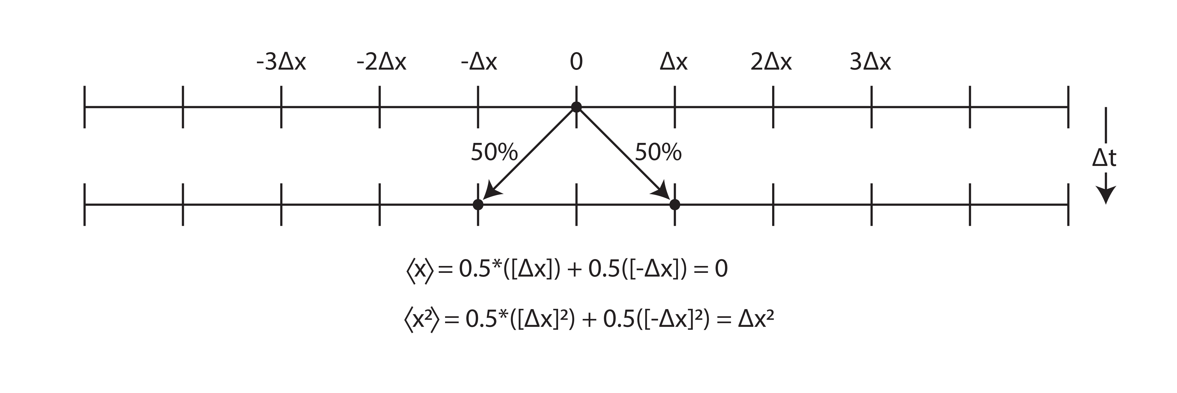
\[\langle x \rangle = \tfrac{1}{2}(-\Delta x) + \tfrac{1}{2}(+\Delta x) = 0.\]
After \(N\) independent steps the total displacement is just the sum of the individual steps,
\[x(t) = \sum_{i=1}^N \Delta x_i = \Delta x_1 + \Delta x_2 + \cdots + \Delta x_N .\]
Now average both sides. The average of a sum is the sum of the averages, so the average can be taken step by step:
\[\langle x(t) \rangle = \langle \Delta x_1 + \Delta x_2 + \cdots + \Delta x_N \rangle = \langle \Delta x_1 \rangle + \langle \Delta x_2 \rangle + \cdots + \langle \Delta x_N \rangle .\]
Every step is drawn from the same symmetric coin flip, so each of those averages is the zero computed just above:
\[\langle x(t) \rangle = \underbrace{0 + 0 + \cdots + 0}_{N \text{ terms}} = 0 .\]
The number of steps never enters the result. Adding more steps only adds more zeros, so the average position stays at the origin however long the particle walks. This is not a claim that the particle stays put: any individual particle randomly moves far from zero. It is a claim about the ensemble, where every particle that drifts right is matched, on average, by one that drifts left. Diffusion spreads a distribution; it does not produce net directed motion.
Mean-squared displacement grows linearly in time
Because the average displacement is zero, the mean-squared displacement \(\langle x^2\rangle\) is a better way to track how far a particle has moved.
At \(t = \Delta t\) (one step):
\[\langle x^2 \rangle = \tfrac{1}{2}(-\Delta x)^2 + \tfrac{1}{2}(+\Delta x)^2 = (\Delta x)^2.\]
At \(t = 2\Delta t\) (two steps):
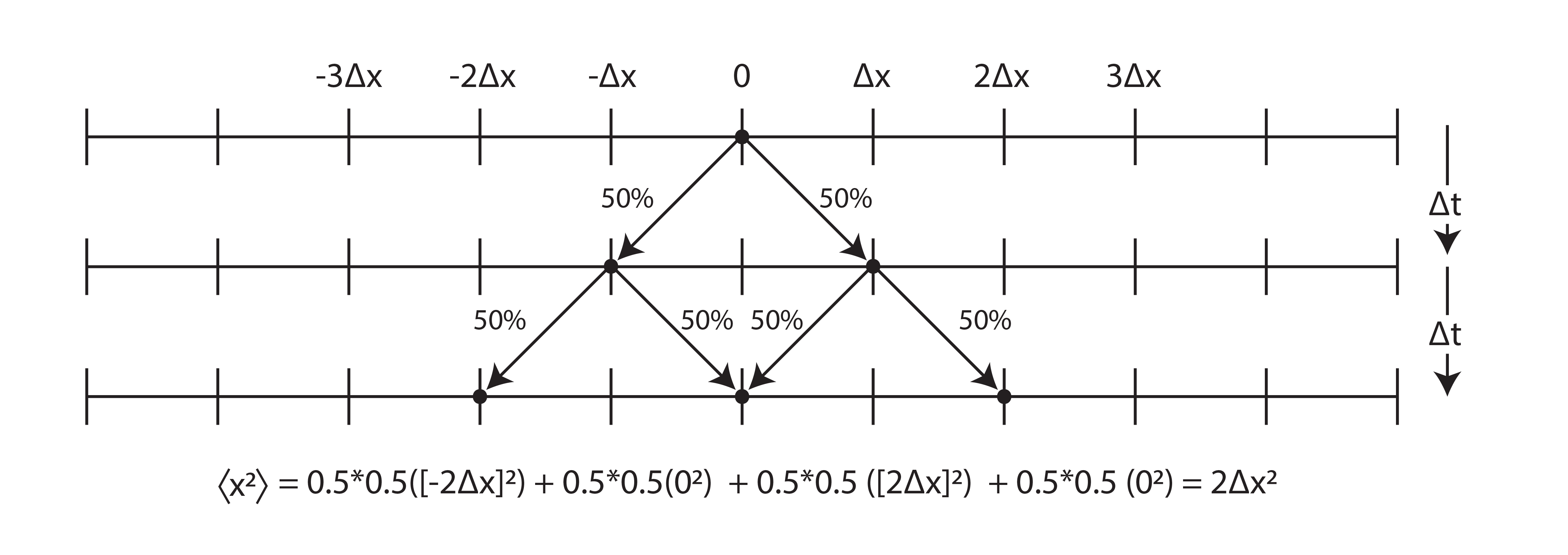
\[\langle x^2 \rangle = \tfrac{1}{4}(-2\Delta x)^2 + \tfrac{1}{2}(0)^2 + \tfrac{1}{4}(2\Delta x)^2 = 2(\Delta x)^2.\]
At \(t = 3\Delta t\) (three steps):
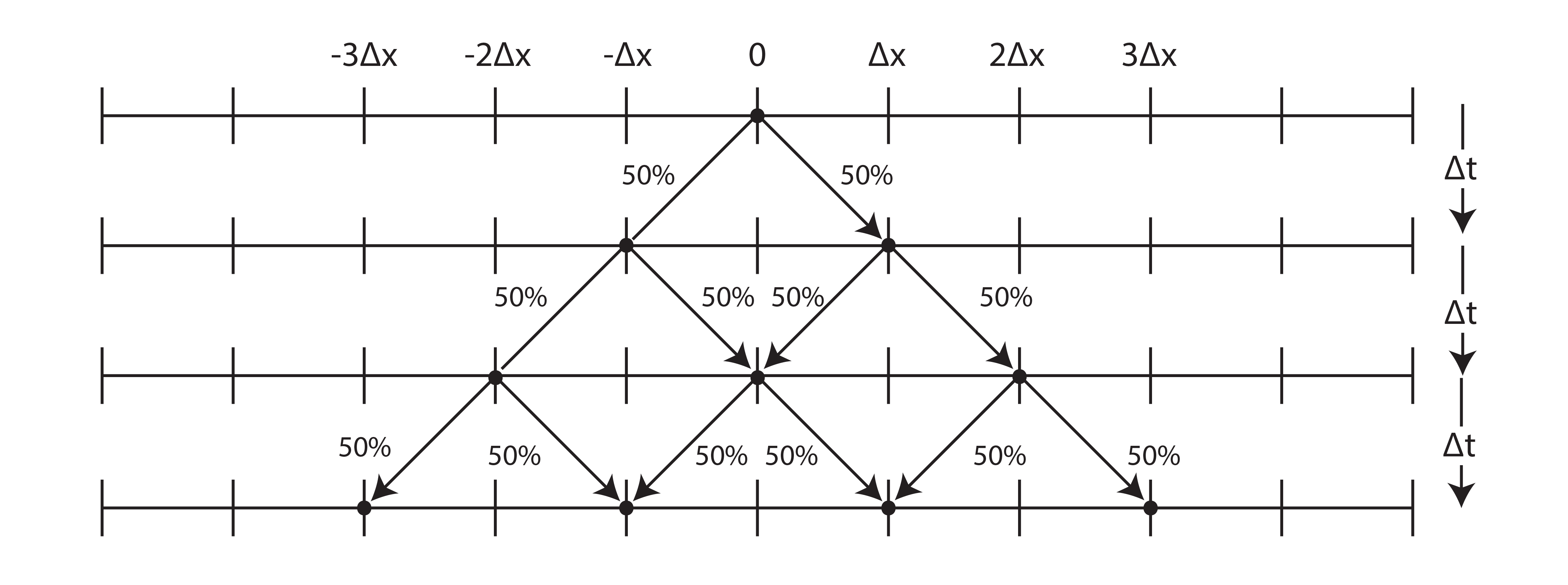
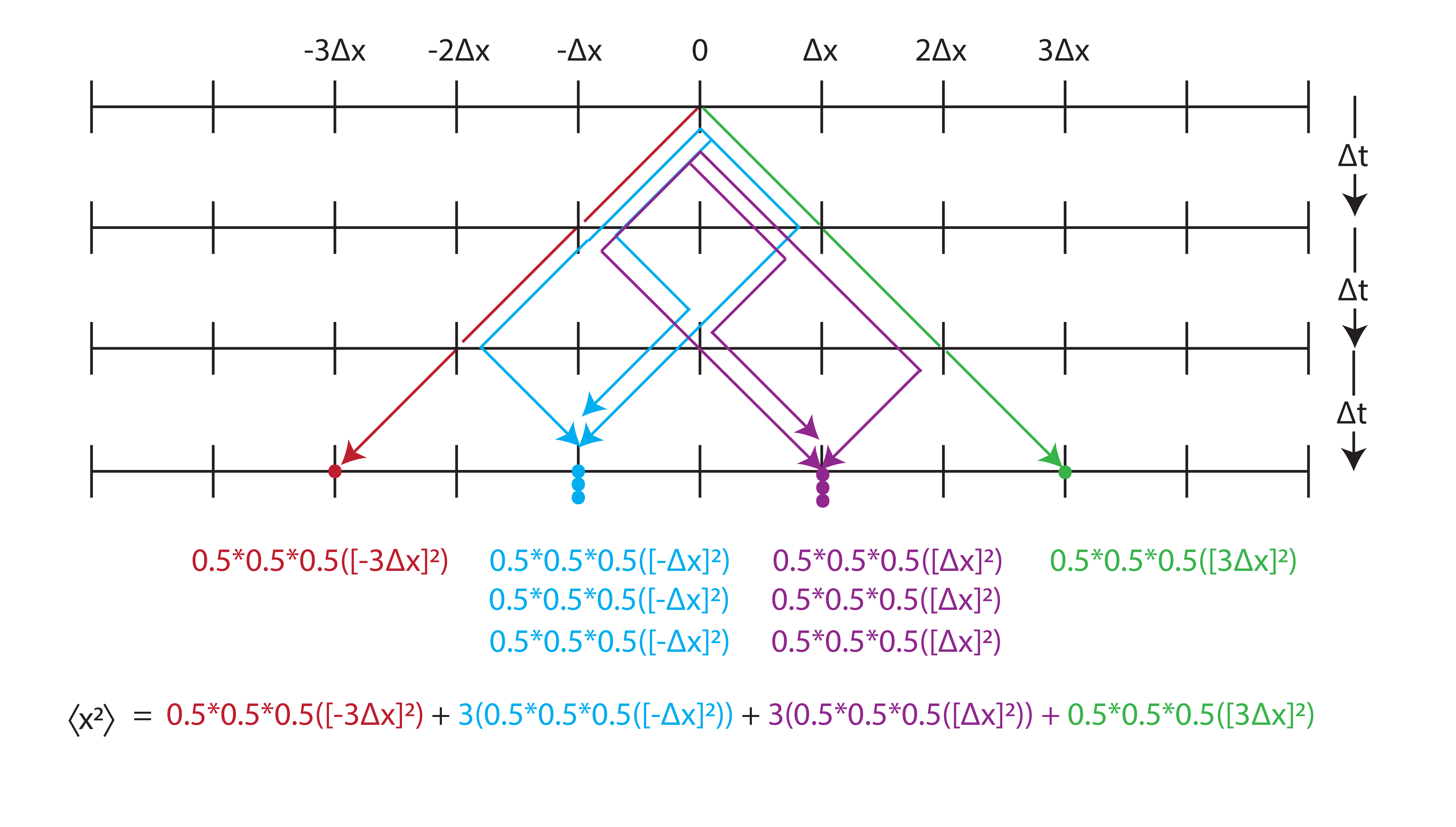
\[\langle x^2 \rangle = 3(\Delta x)^2.\]
The pattern is clear: after \(N\) steps, \(\langle x^2\rangle = N(\Delta x)^2\). Since \(N = t/\Delta t\),
\[\langle x^2(t)\rangle = \frac{t}{\Delta t}(\Delta x)^2.\]
Defining \(D \equiv (\Delta x)^2/(2\Delta t)\) gives the central result of this section:
\[\langle x^2(t)\rangle = 2Dt,\]
where the diffusion coefficient \(D\) has units \(\text{m}^2/\text{s}\). This 1D result generalizes directly to three dimensions: because the \(x\), \(y\), and \(z\) components of a 3D random walk are independent, each contributes \(2Dt\) to the total, giving \(\langle r^2\rangle = 6Dt\). This is a very useful equation because, with only the diffusion coefficient and time, you can calculate the mean-squared displacement.
Physical meaning: square-root growth
The result \(\langle x^2\rangle = 2Dt\) tells us that the root-mean-squared displacement grows as \(\sqrt{t}\):
\[x_{\text{rms}} \equiv \sqrt{\langle x^2\rangle} = \sqrt{2Dt}.\]
Doubling the diffusion time doubles the mean-squared displacement but increases the root-mean-squared distance by only a factor of \(\sqrt{2}\). To double the distance, the time must quadruple. Diffusion is a slow process on long length scales.
For oxygen in water (\(D = 2\times10^{-9}\ \text{m}^2/\text{s}\)) the rms displacement is:
| Time \(t\) | \(x_{\text{rms}} = \sqrt{2Dt}\) |
|---|---|
| \(1\ \text{ms}\) | \(\approx 2\ \mu\text{m}\) |
| \(1\ \text{s}\) | \(\approx 63\ \mu\text{m}\) |
| \(1\ \text{min}\) | \(\approx 490\ \mu\text{m}\) |
| \(1\ \text{h}\) | \(\approx 3.8\ \text{mm}\) |
An oxygen molecule takes about a minute to wander \(\sim 500\ \mu\text{m}\) by diffusion alone, which is why scaffolds must be thin.
Simulating many random walks
import numpy as np
import matplotlib.pyplot as plt

plt.style.use("../../theme/bioe10.mplstyle")   # notebooks run from chapters/<part>/ (cwd), so ../../ = repo root

np.random.seed(42)  # for reproducibility

# ── parameters ────────────────────────────────────────────────────────────────
N_walkers = 1000      # number of independent particles
N_steps   = 500       # number of time steps per walker
dx        = 1.0       # step size in arbitrary units (set D = 1/2)
D         = dx**2 / 2 # diffusion coefficient (units: [dx]^2/step)

# ── simulate ──────────────────────────────────────────────────────────────────
steps   = np.random.choice([-dx, dx], size=(N_walkers, N_steps))
x_traj  = np.cumsum(steps, axis=1)          # (N_walkers, N_steps)
t       = np.arange(1, N_steps + 1)         # time axis in steps

# ensemble-average mean-squared displacement
msd_sim  = np.mean(x_traj**2, axis=0)       # (N_steps,)
msd_theory = 2 * D * t

# ── figure ────────────────────────────────────────────────────────────────────
fig, axes = plt.subplots(1, 2, figsize=(10, 4))

# left: 20 individual trajectories
for i in range(20):
    axes[0].plot(t, x_traj[i], lw=0.6, alpha=0.5, color="#0072B2")
axes[0].set_xlabel("Time step $t$")
axes[0].set_ylabel("Position $x$ (step units)")
axes[0].axhline(0, color="#333333", lw=0.8, ls="--")

# right: MSD vs time — simulation vs theory. Both curves rise from the
# lower-left, so the legend sits in the empty upper-left corner (no overlap).
axes[1].plot(t, msd_sim, color="#0072B2", label="Simulation (ensemble avg.)")
axes[1].plot(t, msd_theory, color="#E69F00", ls="--", lw=1.8, label=r"Theory $\langle x^2\rangle=2Dt$")
axes[1].set_xlabel("Time step $t$")
axes[1].set_ylabel(r"$\langle x^2\rangle$ (step units$^2$)")
axes[1].legend(loc="upper left")

plt.savefig("../../images/02_tissue/random_walk_simulation.png", dpi=150, bbox_inches="tight")
plt.show()

# print key result
print(f"At t = {N_steps} steps: simulated MSD = {msd_sim[-1]:.1f},  theory = {msd_theory[-1]:.1f}")
Running the code prints
At t = 500 steps: simulated MSD = 505.6, theory = 500.0and produces Figure 16.2.
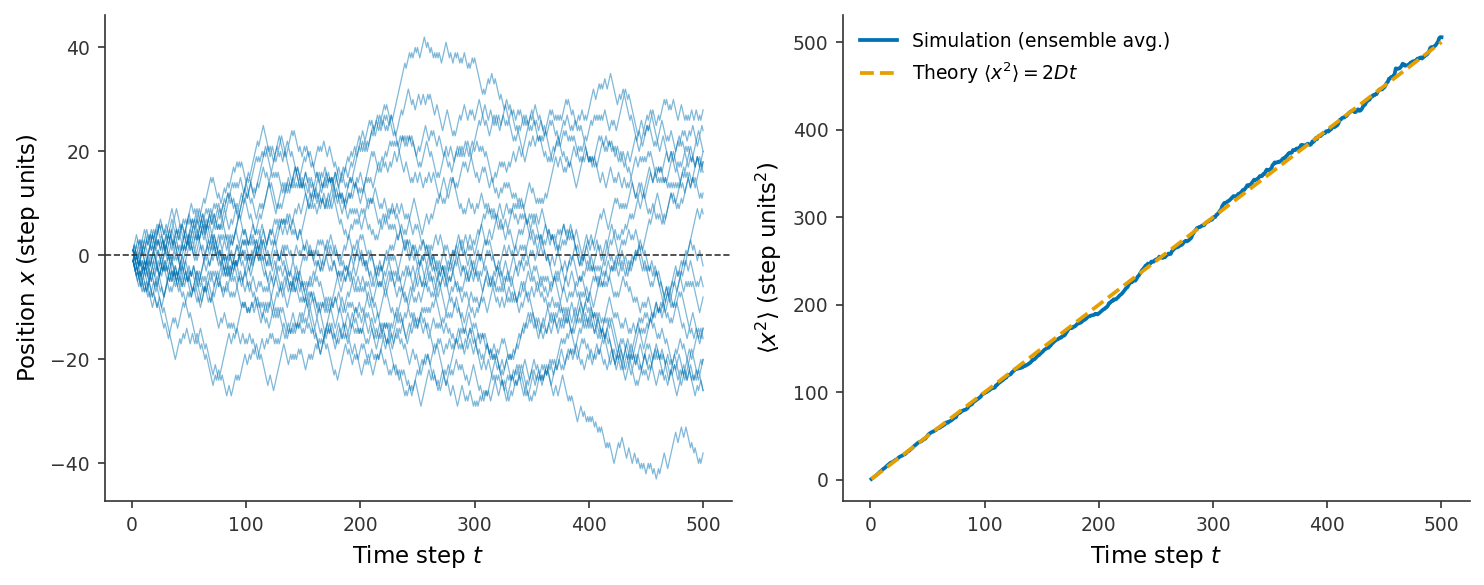
The left panel shows 20 individual random walks, each erratic. The right panel shows the ensemble average of \(1000\) walks: the simulated MSD (blue) closely follows the theoretical prediction \(\langle x^2\rangle = 2Dt\) (orange dashed). The agreement confirms that the simple step-counting derivation above is correct.
The diffusion coefficient connects microscale to macroscale
The result \(D = (\Delta x)^2/(2\Delta t)\) links the microscopic steps to the macroscopic transport constant. In a liquid, \(\Delta x\) and \(\Delta t\) are effective parameters describing the molecule’s motion, and only the combination \((\Delta x)^2/(2\Delta t)\) can be measured: for oxygen in water near room temperature it is \(D \approx 2\times10^{-9}\ \text{m}^2/\text{s}\) (Milo et al. 2010). Larger molecules (proteins, polysaccharides) have smaller \(D\) because their larger radius slows their collisions with solvent molecules; this relationship is quantified by the Stokes–Einstein equation \(D = k_BT/(6\pi\eta r)\), where \(\eta\) is the viscosity of the medium and \(r\) is the hydrodynamic radius, though we will not use that equation in this module.