4 Ultrasound
The instrument used to perform an ultrasound scan of the heart is called an echocardiogram. It is noninvasive, operates in real time, and resolves the chambers contracting and the blood streaming through the valves, all from a probe pressed against the chest (Grogan and Mount 2023). The device that transmits and receives is a transducer: a probe, applied to the skin, that converts an electrical signal into a mechanical vibration — launching the pressure wave — and converts the returning pressure wave back into an electrical signal. It is both source and detector. This section discusses how a pressure wave is transmitted into the body, how its echoes are converted into a measurement of depth, what governs the sharpness of the resulting image, and how a Doppler measurement of blood velocity is obtained from the frequency shift in a returning echo.
The frequency is chosen for a specific engineering purpose. Human hearing spans approximately 20 Hz to 20,000 Hz (20 kHz); ultrasound is defined as any sound above this upper limit, inaudible to the human ear (Grogan and Mount 2023). Medical imaging operates at frequencies in the megahertz range, typically 2 to 10 MHz — hundreds of times higher than the highest audible tone (Grogan and Mount 2023; Aldrich 2007). In soft tissue the speed of sound is fixed at \(c \approx 1540~\text{m/s}\), so \(v = f\lambda\) rearranges to \(\lambda = c/f\), and a megahertz frequency yields a wavelength below one millimeter. Because a wave resolves detail no finer than its own wavelength, the elevated frequency produces a wavelength small enough to resolve important features of the heart.
The code below computes the wavelength across this range, from audible sound to the pulses emitted by an ultrasound probe.
import numpy as np
import matplotlib.pyplot as plt
plt.style.use("../../theme/bioe10.mplstyle")

c = 1540.0                      # speed of sound in soft tissue, m/s

# --- wavelength lambda = c / f, from audible frequencies up to ultrasound ---
points = {"20 Hz": 20, "20 kHz": 20e3, "2 MHz": 2e6, "10 MHz": 10e6}
print("wavelength in soft tissue (c = 1540 m/s):")
for label, f in points.items():
    lam = c / f
    shown = f"{lam*1e3:.3g} mm" if lam < 1 else f"{lam:.3g} m"
    print(f"  {label:>7}  ->  lambda = {shown}")

# --- at a fixed speed, doubling the frequency halves the wavelength ---
f1, f2 = 2e6, 4e6                        # 2 MHz and 4 MHz
lam1, lam2 = c / f1, c / f2
print(f"\n2 MHz -> {lam1*1e3:.3f} mm ;  4 MHz -> {lam2*1e3:.3f} mm "
      f"(doubling f halved lambda)")

fig, (axA, axB) = plt.subplots(1, 2, figsize=(10, 4.2))
Running it prints
wavelength in soft tissue (c = 1540 m/s):
    20 Hz  ->  lambda = 77 m
   20 kHz  ->  lambda = 77 mm
    2 MHz  ->  lambda = 0.77 mm
   10 MHz  ->  lambda = 0.154 mm

2 MHz -> 0.770 mm ;  4 MHz -> 0.385 mm (doubling f halved lambda)
At megahertz frequencies the wavelength falls below a millimeter: a 2 MHz pulse has a wavelength of \(0.77~\text{mm}\), and a 10 MHz pulse just \(0.15~\text{mm}\).
Echoes and acoustic impedance
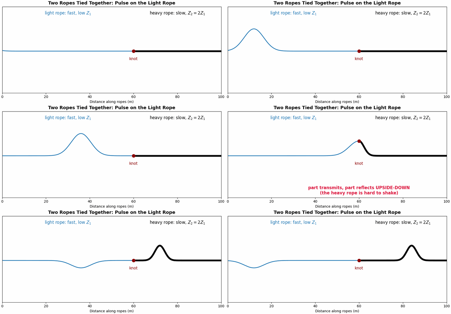
The sound wave reflects off medium that has different properties from the one it is traveling through. The greater the difference, the stronger the reflection. A mechanical analogy may be helpful in understanding this. Imagine tying a light rope to a heavy rope and flicking a pulse into the light one: at the knot where the ropes are connected, part of the pulse continues into the heavy rope (transmitted), and part bounces back along the light rope (reflected), because the heavy rope resists motion almost like a wall (Figure 4.1).
A wave reflects at a boundary where the properties of the medium change, and the property that governs the reflection is the acoustic impedance \(z\). The impedance is the medium’s resistance to being set in motion by the incoming pressure wave. It is the product of the medium’s density \(\rho\) and its speed of sound \(c\) (Urone and Hinrichs 2012):
\[z = \rho\,c .\]
Its units are \(\text{kg}\,\text{m}^{-2}\,\text{s}^{-1}\), also termed the rayl. Impedance combines two properties already assigned to the medium in the waves section. An echo is produced wherever the impedance changes, and the magnitude of the echo increases with the size of the mismatch. When a wave travels from a medium of impedance \(z_1\) into one of impedance \(z_2\), the fraction of the incident intensity reflected at the boundary is (Urone and Hinrichs 2012)
\[R = \left(\frac{z_2 - z_1}{z_2 + z_1}\right)^{2}.\]
When the media are closely matched, \(z_2 \approx z_1\), the numerator approaches zero and \(R \approx 0\): almost no intensity reflects and the wave is transmitted. When the media are strongly mismatched, \(R\) approaches 1 and nearly all the intensity reflects. Table 4.1 lists representative impedances for the body’s tissues, adapted from OpenStax College Physics:
| Medium | Acoustic impedance \(z\) (\(10^{6}~\text{kg}\,\text{m}^{-2}\text{s}^{-1}\)) |
|---|---|
| Air | 0.000429 |
| Fat | 1.34 |
| Blood | 1.66 |
| Soft tissue (average) | ~1.63 |
| Muscle | 1.70 |
| Bone | 5.7 – 7.8 |
Let’s apply the reflection formula to Table 4.1 for a typical ultrasound scan. The soft tissues (fat, blood, muscle) have impedances that differ only slightly, so the boundaries between them reflect only about one percent of the wave. This weak reflection is the essential feature rather than a limitation: because most of the wave is transmitted at each soft-tissue boundary, the pulse penetrates further and retains sufficient intensity to echo off successive structures. A small fraction reflects at each interface, enough to register it, while the remainder continues onward. This is why a blood–tissue boundary — the inner surface of a heart chamber, the edge of a valve leaflet — appears on an echocardiogram: blood (\(1.66\)) against muscle (\(1.70\)) is a small but genuine mismatch that can be rendered as a bright line.
Air has an impedance thousands of times smaller than tissue, so a tissue–air boundary reflects about 99.9% of the wave, an almost total reflection. A thin layer of air trapped between the probe and the skin would therefore transmit essentially none of the wave into the body. To avoid this, coupling gel is applied to exclude the air and replace the tissue–air interface with a tissue–gel match through which the wave can pass. At the other extreme, bone has an impedance several times that of soft tissue, so a tissue–bone boundary reflects a large fraction of the wave; bones and calcifications appear bright and cast an acoustic shadow behind them. This is one reason the probe for a cardiac scan is angled to image between the ribs rather than through them.
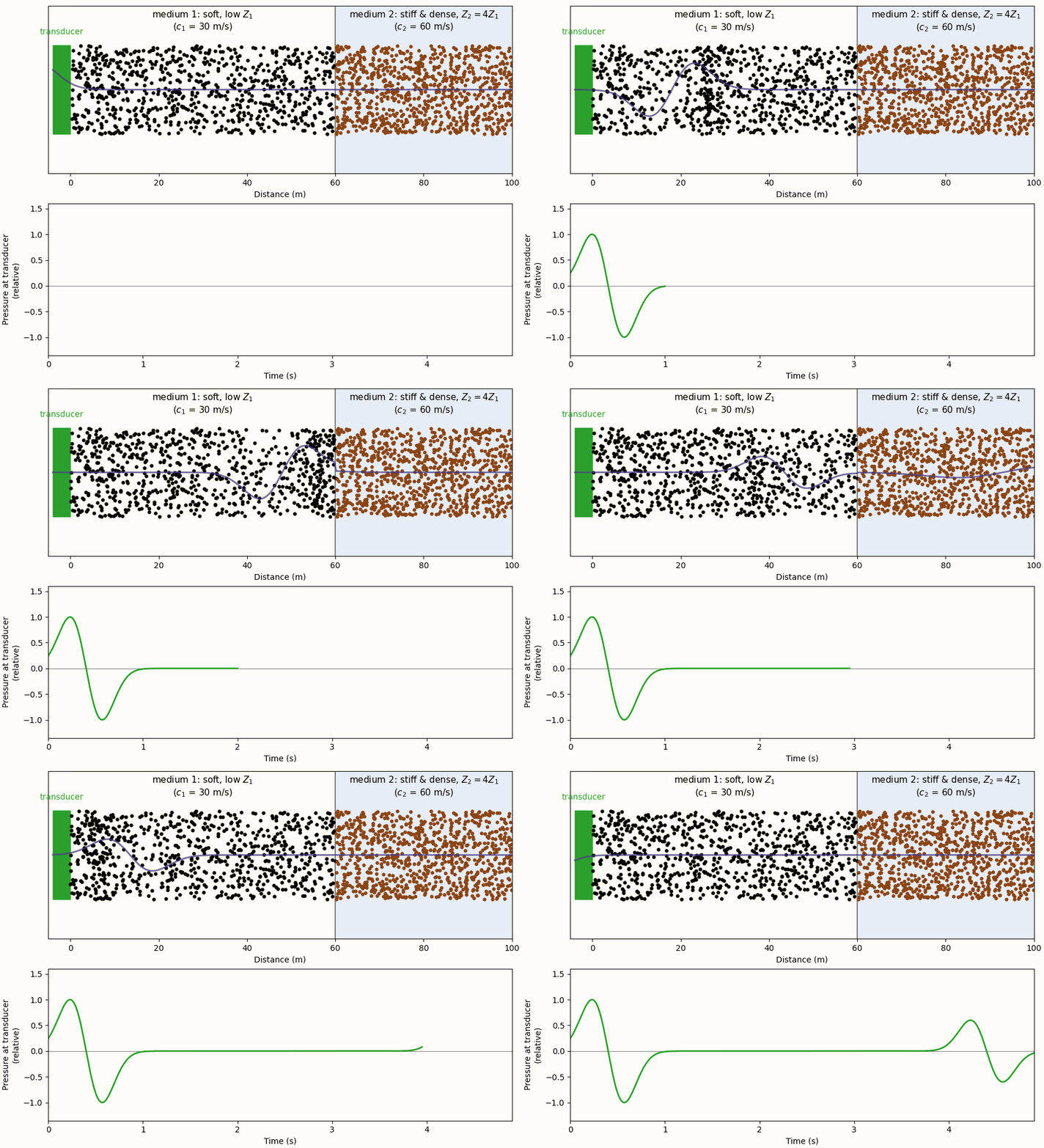
The device that transmits and receives is a transducer: a probe, applied to the skin, that converts an electrical signal into a mechanical vibration that launches a pressure wave. It also converts the returning pressure wave back into an electrical signal. It is both source and detector. Figure 4.2 simulates a transducer firing a pulse across exactly such a boundary, with an impedance ratio \(Z_2 = 4Z_1\) comparable to tissue against bone, and records what the transducer sees.
Depth from timing
The transducer sends a pulse and records the echo, measuring the time \(t\) it takes to return. Because the pulse travels to the reflecting structure and back at the known tissue speed \(c \approx 1540~\text{m/s}\), the round-trip time can be converted directly into a distance. The pulse traverses a total path \(c\,t\), and the structure lies at half that distance:
\[d = \tfrac{1}{2}\,c\,t .\]
The factor of one-half reflects the round trip: the echo traverses twice the depth, so the depth is half the total path. A structure twice as deep returns its echo twice as late (Figure 4.3). The transducer transmits a pulse and then receives; each interface the pulse crosses returns a faint echo, and the arrival time of each echo encodes the depth of the interface that produced it.
import numpy as np

c = 1540.0                 # speed of sound in soft tissue, m/s
d1, d2 = 0.05, 0.12         # interface depths, m (5 cm and 12 cm)
t1, t2 = 2 * d1 / c, 2 * d2 / c    # round-trip time to each interface, t = 2d/c
# ... simulate a short windowed-sinusoid pulse at t=0, t1, and t2, and plot the
# summed trace against time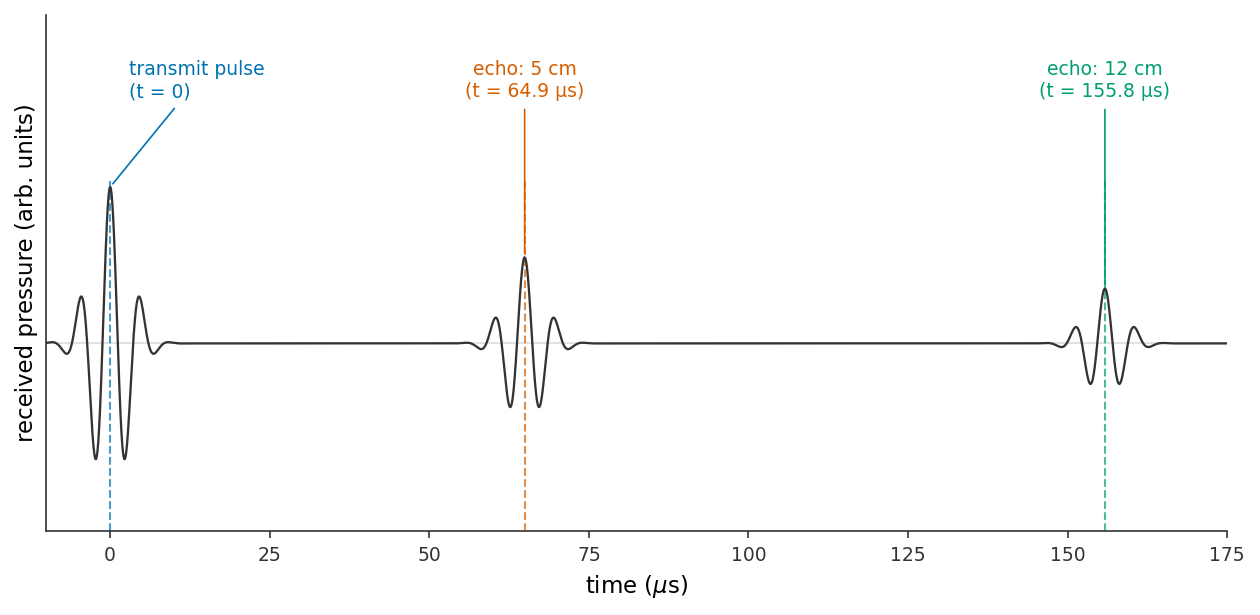
A pulse and its sequence of timed echoes, constitutes one line of an image: a profile of the structures directly beneath the probe at every depth along the beam. An echocardiogram is assembled by sweeping the beam across the heart and stacking many such lines into a two-dimensional image updated tens of times per second. The mechanism by which the scanner steers and combines these lines (beamforming and image reconstruction) is beyond the present scope of this text.
An ultrasound scanner locates a structure by timing its echo. With the tissue speed of sound \(c \approx 1540~\text{m/s}\) fixed and known, a round-trip time \(t\) places the reflector at a depth
\[\boxed{\; d = \tfrac{1}{2}\,c\,t \;}\]
the factor of one-half arising because the pulse travels out and back. Many such timed lines, placed side by side, compose an image.
The imaging trade-off: resolution versus penetration
Resolution and penetration depend on frequency in opposing directions. Raising the frequency sharpens the image but reduces the depth to which the wave penetrates. The choice of frequency is therefore a compromise between the desired resolution and the required penetration depth.
Consider resolution first. A wave resolves detail approximately as fine as its wavelength, so the finest structure a beam can distinguish along its direction of travel — its axial resolution — improves as the wavelength decreases. Since \(\lambda = c/f\) at fixed tissue speed, higher frequency yields shorter wavelength and finer detail. A 3 MHz pulse has \(\lambda \approx 0.5~\text{mm}\); a 7.5 MHz pulse has \(\lambda \approx 0.2~\text{mm}\), resolving features two and a half times smaller.
Consider penetration second. As a pressure wave travels through tissue it is steadily attenuated (its energy absorbed and scattered), and the attenuation increases with frequency, at a rate of roughly \(0.5~\text{dB}\) per centimeter per megahertz (Grogan and Mount 2023; Aldrich 2007). A high-frequency pulse is sharp but shallow, decaying within a few centimeters; a low-frequency pulse is coarser but reaches further.
import numpy as np

c = 1540.0                      # speed of sound in soft tissue, m/s

for f in (3e6, 7.5e6):          # a deep cardiac probe vs a superficial vascular probe
    lam = c / f                 # wavelength = axial-resolution scale
    penetration = 500 * lam     # effective imaging depth, rule of thumb ~500 wavelengths
    print(f"f = {f/1e6:4.1f} MHz  ->  lambda = {lam*1e3:5.3f} mm ,"
          f"  penetration ~ {penetration*100:4.1f} cm")
which prints
f =  3.0 MHz  ->  lambda = 0.513 mm ,  penetration ~ 25.7 cm
f =  7.5 MHz  ->  lambda = 0.205 mm ,  penetration ~ 10.3 cm
import numpy as np
import matplotlib.pyplot as plt
plt.style.use("../../theme/bioe10.mplstyle")
c = 1540.0 # speed of sound in soft tissue, m/s
f = np.linspace(1e6, 15e6, 400) # diagnostic band, 1-15 MHz
lam = c / f # wavelength = axial-resolution scale
penetration = 500 * lam # effective imaging depth, rule of thumb
# ... plot lambda vs. f (left) and penetration vs. f (right), marking the
# 3 MHz and 7.5 MHz probes from the printed values above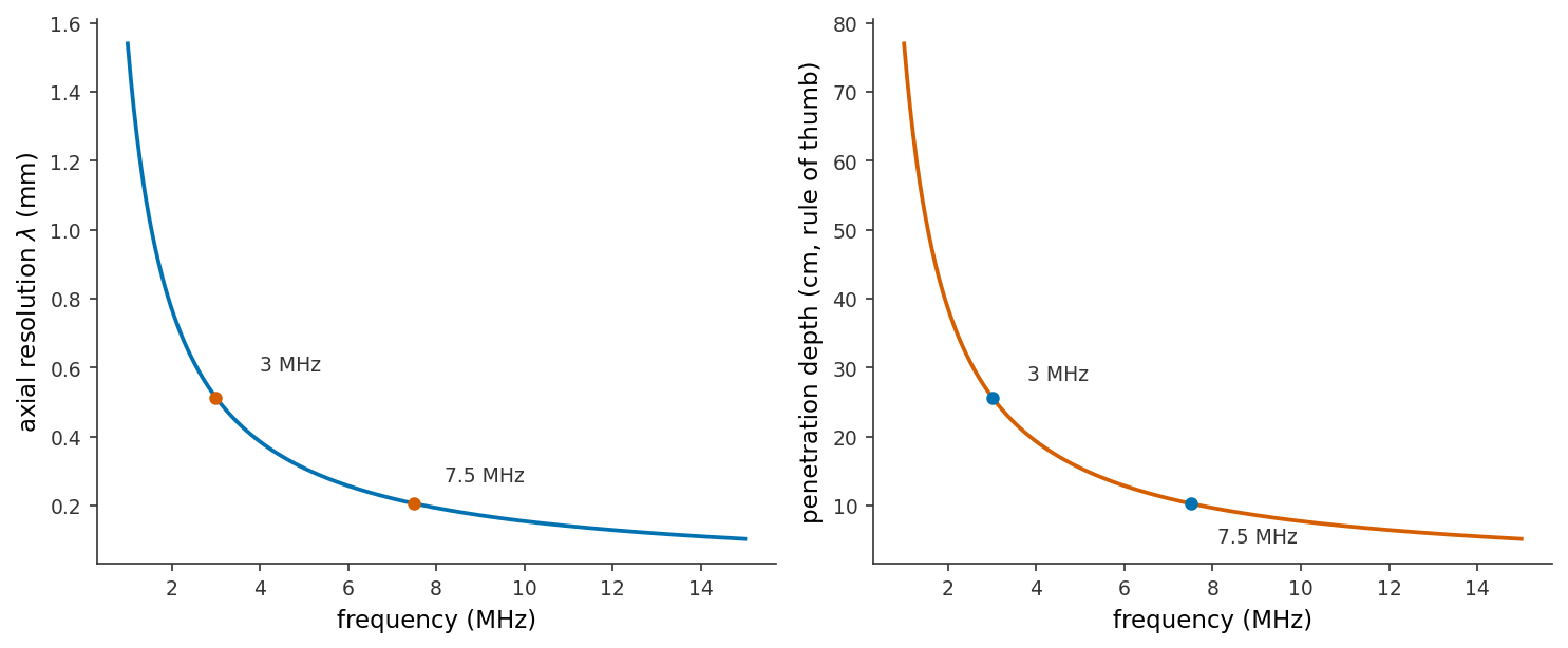
The choice of frequency is therefore effectively a choice of depth. To image the heart, several centimeters within the chest, an echocardiogram uses a low-frequency probe near 2–3 MHz and accepts coarser detail as the cost of that depth. To image a blood vessel or tendon immediately beneath the skin, a probe of 7–15 MHz provides fine detail without requiring substantial reach (Figure 4.4).
Doppler: measuring blood velocity from a frequency shift
The methods so far image structure — the location walls and valves. However, echocardiography can also measure the speed of the blood itself, by the Doppler effect.
The Doppler effect is the shift in the observed frequency of a wave when its source or observer is in motion: motion toward the observer compresses the waves to a higher frequency, and motion away stretches them to a lower one. The pitch of a passing ambulance siren, rising on approach and falling on recession, is the familiar illustration. The same effect applies to an ultrasound pulse reflected from a moving target, and blood presents many such targets in the red cells streaming through a valve. When the beam is directed at blood moving toward the probe, the echo returns at a slightly higher frequency than transmitted, and the magnitude of this Doppler shift \(f_D\) is a direct measure of the blood’s speed.
The moving blood produces the shift twice, once as a receiver and once as a source.
Take a red blood cell moving straight along the beam, toward the probe, at speed \(v\), with the probe transmitting frequency \(f_0\) and tissue sound speed \(c\).
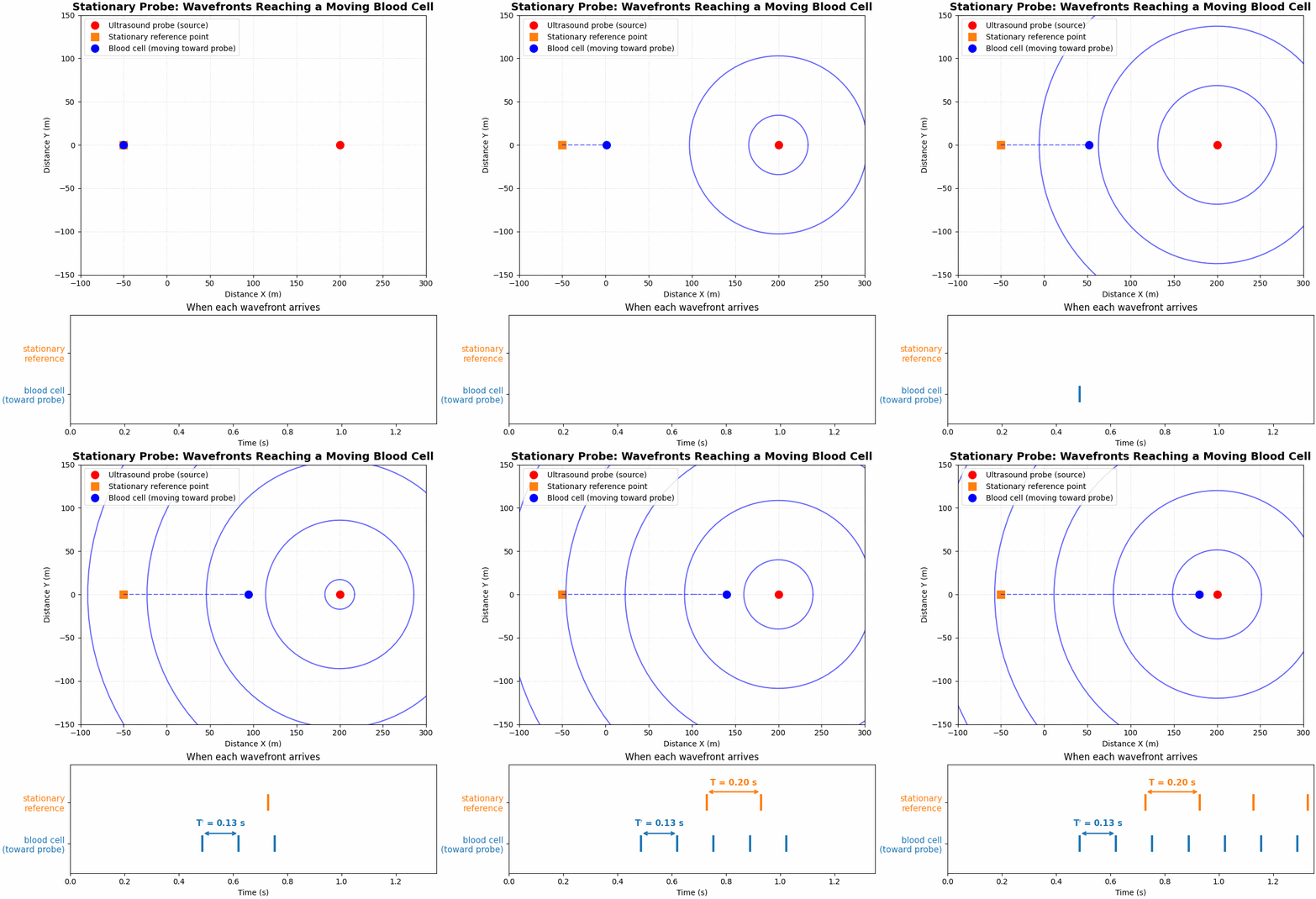
Stage 1 — the cell is a moving receiver. Figure 4.5 shows the general case: a moving observer closes in on wavefronts that a stationary source emits at the ordinary wavelength \(\lambda = c/f_0\). Because the observer meets each successive front sooner than a stationary one would, it receives wavefronts at an elevated rate,
\[f_1 = \frac{c+v}{\lambda} = f_0\,\frac{c+v}{c}.\]
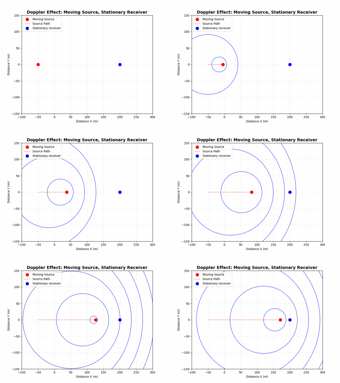
Stage 2 — the cell is a moving source. Having absorbed the beam at frequency \(f_1\), the cell immediately re-emits it as an echo, and it does so while still advancing toward the probe. Figure 4.6 shows what a moving source does to the waves it emits: each successive wavefront is launched from a point closer to the probe than the last, compressing them into a shorter wavelength ahead of the source,
\[\lambda_2 = (c-v)\,T_1 = \frac{c-v}{f_1}, \qquad\text{so the probe receives}\qquad f_2 = \frac{c}{\lambda_2} = f_1\cdot\frac{c}{c-v}.\]
Combining the two stages. Substituting \(f_1\) from Stage 1 into \(f_2\) gives the frequency the probe finally records,
\[f_2 = f_0\,\frac{c+v}{c-v},\]
so the total shift is
\[\Delta f = f_2 - f_0 = f_0\left(\frac{c+v}{c-v}-1\right) = f_0\,\frac{2v}{c-v}.\]
Blood speeds are a few meters per second against a tissue sound speed of \(c\approx1540~\text{m/s}\), so \(v\ll c\) and the small \(v\) in the denominator may be dropped, leaving \(\Delta f \approx 2f_0 v/c\): each stage contributes a shift of \(f_0v/c\), and the two add.
For a beam that meets the blood’s motion at an angle \(\theta\), only the velocity component along the beam, \(v\cos\theta\), contributes to either stage, giving the general result (Urone and Hinrichs 2012)
\[f_D = \frac{2 f_0\, v \cos\theta}{c},\]
where:
- \(f_0\) — the transmitted frequency
- \(c\) — the tissue sound speed
- \(\theta\) — the angle between the beam and the blood’s direction of travel
The factor \(\cos\theta\) enters because only the velocity component along the beam compresses the waves; the shift is largest when the beam is aligned with the jet, \(\theta \approx 0\) and \(\cos\theta \approx 1\). Alignment therefore matters in practice: a beam offset by an unmeasured angle \(\theta\) is treated as aligned (\(\cos\theta \approx 1\)), so the machine reports \(v\cos\theta\), an under-estimate of the true speed. At \(\theta = 60^\circ\), \(\cos\theta = 0.5\) and the reported speed is halved, which is why a sonographer aligns the beam with the jet. Rearranging the relation gives the velocity, the quantity otherwise inaccessible:
\[v = \frac{c\, f_D}{2 f_0 \cos\theta}.\]
The frequency shift of the returning echo thus yields the blood’s speed. For a cardiac probe at \(f_0 = 2~\text{MHz}\) and a fast valve jet, \(f_D\) evaluates to a few kilohertz, within the audible range. The machine plays the Doppler shift through a loudspeaker, and the clinician hears the blood velocity as a tone whose pitch tracks the flow. The heart section began by listening to the heart with a stethoscope; the Doppler method renders a different quantity audible — the measured velocity itself.
A velocity alone is not yet a diagnosis: the quantity that indicates whether a valve is dangerously narrowed is the pressure difference the heart must generate to drive blood through it, and reaching pressure from this velocity requires two further conservation laws, taken up in the sections that follow.
- Ultrasound is a high frequency pressure wave (≈2–10 MHz) designed so that its sub-millimeter wavelength can resolve anatomy; a transducer both transmits the pulse and receives its echoes.
- Echoes come from impedance mismatches. With \(z = \rho c\), the reflected fraction is \(R = \big((z_2-z_1)/(z_2+z_1)\big)^2\): soft-tissue boundaries reflect weakly (so the pulse sees deep), while air and bone reflect strongly (hence coupling gel and acoustic shadows).
- Depth comes from timing, \(d = \tfrac{1}{2}ct\); stacking timed lines makes an image.
- Resolution and penetration trade off. Higher frequency \(\to\) shorter \(\lambda\) \(\to\) finer detail, but \(\to\) more attenuation \(\to\) shallower reach.
- Doppler measures velocity. The echo’s frequency shift gives the blood-jet velocity, \(v = c f_D / (2 f_0 \cos\theta)\) — the quantity the sections that follow convert into the valve pressure gradient.