25 Numerical Data
Data types split variables into two types: numerical and categorical. For a numerical variable, the distribution can be visualized, and its center and spread can be described.
Histograms
The distribution of a variable describes the values it takes, together with how often each occurs. For a numerical variable, this distribution is often represented with a histogram.
Consider 200 glucose readings from a continuous sensor worn by one hypothetical participant over about a day, each in mg/dL. Each reading is one value, and the set of readings is a dataset.
A list of the values does not show their shape (see Figure 25.1). For a numerical variable, how often each range of values occurs is found by binning: the number line is split into intervals called bins, and the values in each bin are counted. A histogram draws a bar above each bin, with height equal to how many values fell there.
rng = np.random.default_rng(21)
base = rng.lognormal(np.log(92), 0.12, size=170)     # fasting and between-meal readings
peak = rng.lognormal(np.log(150), 0.18, size=30)     # post-meal peaks
glucose = np.round(np.concatenate([base, peak]), 0)
rng.shuffle(glucose)
fig, ax = plt.subplots(figsize=(7, 2.2))
ax.vlines(glucose, 0, 1, color=BLUE, alpha=0.5, lw=1)     # one line per reading
ax.set_ylim(0, 1)
ax.set_yticks([])
ax.set_xlabel("glucose reading (mg/dL)")
plt.show()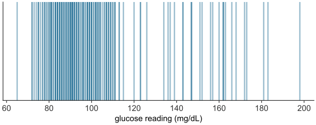
scripts/03_statistics/04_numerical_data/gen_numerical_data.py.
The bins must be contiguous and drawn to scale on the number line, so position and width carry meaning. A value landing exactly on a boundary needs a rule. By convention each bin includes its left endpoint and excludes its right, written \([a, b)\), so a value equal to \(b\) belongs to the next bin up.
Constructing a histogram from continuous data
A glucose reading, in \(\text{mg/dL}\), is continuous: between any two readings, however close, another is possible. The analyst therefore has to choose the bin width.
Take the \(200\) readings. Plot each reading as a dot on the number line, positioned at its value, then stack the dot above the \(10\ \text{mg/dL}\)-wide bin that contains it (see Figure 25.2). Once the readings are placed, the height of each stack is the bar a histogram draws over that bin.
rng = np.random.default_rng(21)
base = rng.lognormal(np.log(92), 0.12, size=170)     # fasting and between-meal readings
peak = rng.lognormal(np.log(150), 0.18, size=30)     # post-meal peaks
glucose = np.round(np.concatenate([base, peak]), 0)
rng.shuffle(glucose)
print(f"glucose (mg/dL): min {glucose.min():.0f}   median {np.median(glucose):.1f}   max {glucose.max():.0f}")

glu_bins = np.arange(60, 231, 10)                    # 10 mg/dL bins
bin_of_reading = np.digitize(glucose, glu_bins) - 1
PER_ROW = 5                                          # dots laid side by side within each bin

fig, ax = plt.subplots()
ax.hist(glucose, bins=glu_bins, color=BLUE, alpha=0.3, edgecolor=BLUE)   # the bars the stacks will match
slot = np.zeros(len(glu_bins) - 1, dtype=int)        # next open row-and-column in each bin's stack
for i in np.argsort(glucose):                        # place the lowest reading first, then the next...
    b = bin_of_reading[i]
    k = slot[b]
    x = glu_bins[b] + 1 + 8 * (k % PER_ROW + 0.5) / PER_ROW
    y = PER_ROW * (k // PER_ROW) + PER_ROW / 2
    ax.plot(x, y, "o", color=BLUE)                 # one dot per reading
    slot[b] += 1
ax.set_xlabel("glucose reading (mg/dL)")
ax.set_ylabel("number of readings")
plt.show()
glucose (mg/dL): min 65 median 93.5 max 198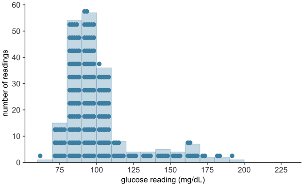
scripts/03_statistics/04_numerical_data/gen_numerical_data.py.
Too wide, and bins swallow real structure: a single bin from \(60\) to \(130\) mg/dL would report that most readings are ordinary, erasing the difference between a reading of \(80\) and one of \(120\). Too narrow, and most bins hold one or two readings each, so bar heights no longer reflect the distribution’s shape. The \(10\ \text{mg/dL}\) width used here suits this dataset; it is not a rule.
The histogram in depth: shape and the density scale
The values run from \(65\) to \(198\) mg/dL. Binning them in intervals of \(10\) mg/dL gives the histogram (see Figure 25.3).
rng = np.random.default_rng(21)
base = rng.lognormal(np.log(92), 0.12, size=170)     # fasting and between-meal readings
peak = rng.lognormal(np.log(150), 0.18, size=30)     # post-meal peaks
glucose = np.round(np.concatenate([base, peak]), 0)
rng.shuffle(glucose)
print("glucose (mg/dL):")
print(f"  min {glucose.min():.0f}   median {np.median(glucose):.1f}   "
      f"mean {glucose.mean():.1f}   max {glucose.max():.0f}")

fig, ax = plt.subplots()
ax.hist(glucose, bins=np.arange(60, 231, 10), color=BLUE, edgecolor="white")
ax.set_xlabel("glucose reading (mg/dL)")
ax.set_ylabel("number of readings")
plt.show()
glucose (mg/dL):
min 65 median 93.5 mean 100.9 max 198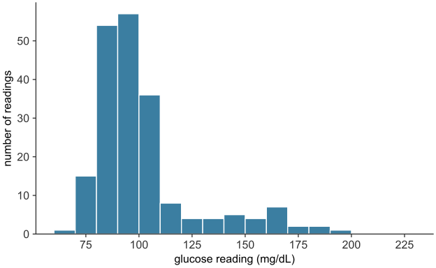
scripts/03_statistics/04_numerical_data/gen_numerical_data.py.
More than half of the readings fall between \(80\) and \(100\) mg/dL, and a long, thin tail stretches to the right. The tail is made of post-meal peaks, readings well above the fasting range. A distribution of this form is called right-skewed, or skewed toward high values. It is common wherever a quantity is bounded below but can occasionally run very large: incomes, city populations, blood concentrations after a dose.
A distribution with a long, thin tail to the left is called left-skewed. One that trails off about equally in both directions is symmetric.
A reading of exactly \(100\) mg/dL falls in the bin \([100, 110)\), not \([90, 100)\), since each bin holds its left edge. Because the sensor reports whole numbers, \(23\) of the \(200\) readings fall exactly on a bin edge.
Both draw bars over a distribution, but they are not interchangeable.
- A bar chart displays a categorical distribution (categorical data). Its bars have equal width, stand apart with gaps, and may be placed in any order; only their lengths carry information.
- A histogram displays a numerical distribution. Its bars are contiguous and positioned to scale on a number line, so that their widths and positions carry information; the bars may not be reordered.
Using one where the other belongs (a histogram of blood types, a bar chart of glucose readings with the bars rearranged) misrepresents the data.
The vertical axis: counts and the density scale
The height of each bar is a raw count, the number of readings in the bin. That reads correctly here only because the bins share one width, \(10\) mg/dL, so a taller bar holds more readings. Two situations break this. When bins have unequal widths, a wide bin accumulates more values simply by covering more ground. And when two distributions built from different numbers of individuals are compared, the larger dataset posts taller bars everywhere, regardless of shape. The remedy in both cases is the density scale, on which each bar’s area, not its height, represents the proportion of data in the bin. The height is set to
\[\text{height} = \frac{\text{proportion of values in the bin}}{\text{width of the bin}},\]
so that each bar’s area (height \(\times\) width) equals the proportion of values it contains, and the areas of all the bars sum to \(1\). Densities and areas are then comparable across bin widths and across datasets of any size. In matplotlib, passing density=True to hist performs this normalization.
The center of a distribution
Descriptive statistics reduces a whole distribution to several numbers: a single value for its center and a single value for its spread.
A measure of center is a single value chosen to stand in for an entire distribution, the one number to report when a single value is required. The two most common are the mean and the median.
The mean
The mean (arithmetic mean, or average) of a numerical variable is the sum of its values divided by their count. For values \(x_1, x_2, \ldots, x_n\),
\[ \bar{x} \;=\; \frac{1}{n}\sum_{i=1}^{n} x_i, \]
read “x-bar,” where \(n\) is the number of values, \(x_i\) is the \(i\)-th value, and \(\sum\) denotes their sum. Mechanically, the mean is the value each individual would take if the total were shared out equally. Physically, it is the balance point of the distribution: place a unit weight at each value along the number line, and the mean is the point at which the arrangement would balance. Every value enters the sum, so the mean uses all of the data. And because it balances, moving any single value further out drags the balance point toward it: the mean is sensitive to extreme values.
The median
The median is the middle value of the distribution once the values are sorted: the value with as many observations above it as below. For an odd number of values it is the single middle one; for an even number it is, by convention, the average of the two middle values. Equivalently, the median is the 50th percentile, the point below which half the data falls.
Where the mean weighs the values, the median counts them. It depends on the order of the observations and the identity of the middle one, not on how far the extremes reach: doubling the largest value in a dataset leaves the median untouched. The median is therefore resistant (or robust) to outliers, where the mean is sensitive.
Which to prefer: skew and robustness
The glucose readings form a right-skewed distribution: a dense cluster of ordinary readings and a thin tail of post-meal peaks. For such a distribution, the mean and the median differ. A sensor fault that records the top reading as \(500\) mg/dL instead of \(198\) shows how each summary responds.
mean_g, median_g = glucose.mean(), np.median(glucose)
print(f"mean   = {mean_g:6.1f} mg/dL")
print(f"median = {median_g:6.1f} mg/dL")

faulty = glucose.copy()
faulty[np.argmax(faulty)] = 500                     # sensor fault: top reading recorded as 500
print("\nafter a sensor fault records the top reading as 500:")
print(f"  mean   {mean_g:6.1f} -> {faulty.mean():6.1f}   (moved {faulty.mean() - mean_g:.1f})")
print(f"  median {median_g:6.1f} -> {np.median(faulty):6.1f}   (moved {np.median(faulty) - median_g:.1f})")

fig, ax = plt.subplots()
ax.hist(glucose, bins=np.arange(60, 231, 10), color=BLUE, edgecolor="white")
ax.axvline(median_g, color=GOLD, lw=2.5, label=f"median = {median_g:.1f}")
ax.axvline(mean_g,   color=GOLD, lw=2.5, ls="--", label=f"mean = {mean_g:.1f}")
ax.set_xlabel("glucose reading (mg/dL)")
ax.set_ylabel("number of readings")
ax.legend()
plt.show()
mean = 100.9 mg/dL
median = 93.5 mg/dL
after a sensor fault records the top reading as 500:
mean 100.9 -> 102.4 (moved 1.5)
median 93.5 -> 93.5 (moved 0.0)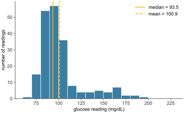
scripts/03_statistics/04_numerical_data/gen_numerical_data.py.
The median, \(93.5\) mg/dL, sits in the main body of the distribution, where a typical reading lies. The mean, \(100.9\) mg/dL, is pulled \(7.4\) mg/dL to the right of it, toward the tail, by the post-meal peaks, even though about two-thirds of the readings fall below that mean (see Figure 25.4). For a skewed distribution, the mean is dragged toward the long tail while the median stays in the body, so the median is usually the more representative center. For a roughly symmetric distribution the two nearly coincide, and either serves. The difference between them is itself a diagnostic: a mean well above the median signals right skew, a mean well below it signals left skew. Despite the median’s robustness, inference is built on the mean, because its algebra is tractable and the median’s is not. The sampling distribution and the hypothesis test need two properties of the mean: it combines additively across groups, and its behavior from sample to sample can be predicted in closed form.
A third measure, the mode (the most frequent value, or equivalently the tallest bar of a histogram), completes the standard set. It is the only measure of center available for a nominal categorical variable, where mean and median are both undefined: there is no average or middle blood type, but there is a most common one. For numerical data the mode sees less use, since it is unstable for continuous measurements, where exact repeats are rare and its value depends on the binning.
The spread of a distribution
Two distributions can share a center yet differ in how tightly their values cluster around it. Consider two treatments with the same mean improvement but different consistency: one moves nearly every patient close to the average, the other produces large gains in some patients and none in others. Reporting the common mean alone would call them equivalent. A measure of spread (or dispersion, or variability) quantifies how far a distribution’s values typically lie from its center.
rng = np.random.default_rng(1)
mu = 20.0

def group_with(sd, n=400):
    # draw n values, then rescale to have mean exactly mu and SD exactly sd
    z = rng.normal(size=n)
    return mu + sd * (z - z.mean()) / z.std(ddof=0)

tight = group_with(2.0)   # treatment A: small spread
wide  = group_with(6.0)   # treatment B: large spread
print(f"treatment A:  mean {tight.mean():.2f}   SD {tight.std(ddof=0):.2f}")
print(f"treatment B:  mean {wide.mean():.2f}   SD {wide.std(ddof=0):.2f}")

lo, hi = min(tight.min(), wide.min()), max(tight.max(), wide.max())
bins = np.linspace(lo, hi, 21)          # common bins, so the overlay is fair
fig, ax = plt.subplots()
ax.hist(tight, bins=bins, density=True, alpha=0.6, color=BLUE,
        edgecolor="white", label="treatment A  (SD = 2)")
ax.hist(wide, bins=bins, density=True, alpha=0.6, color=GOLD,
        edgecolor="white", label="treatment B  (SD = 6)")
ax.axvline(mu, color="black", lw=1.5, ls=":", label="common mean = 20")
ax.set_xlabel("improvement score")
ax.set_ylabel("proportion per unit (density)")
ax.legend()
plt.show()
treatment A: mean 20.00 SD 2.00
treatment B: mean 20.00 SD 6.00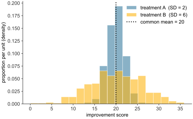
scripts/03_statistics/04_numerical_data/gen_numerical_data.py.
Both groups would be reported as “mean improvement \(20\),” yet their standard deviations are \(2\) and \(6\) points. Treatment A’s results sit close to \(20\); treatment B’s extend further on either side (see Figure 25.5).
Deviations, and why they are squared
Spread is built from the deviation of each value from the mean, \(x_i - \bar{x}\): positive for values above the mean, negative for those below, and larger in magnitude the further out a value lies. Averaging the deviations is the natural first attempt, and it fails: the deviations of any dataset sum to zero, so their average is zero, whatever the spread. The cancellation follows from the mean’s role as balance point, where the positive and negative deviations offset exactly. The signs must therefore be removed before the deviations can be combined into a measure of size.
Two operations remove the sign: take the absolute value \(|x_i - \bar{x}|\), or take the square \((x_i - \bar{x})^2\). Averaging the absolute deviations gives the mean absolute deviation, a measure of spread. The standard choice, however, squares them.
The median plays the matching role for absolute deviations: the value \(c\) that minimizes \(\sum_i |x_i - c|\) is the median.
Variance and standard deviation
The variance is the mean of the squared deviations, the average squared distance from the mean. For a complete population of values \(x_1, \ldots, x_N\) with mean \(\mu\),
\[ \sigma^2 \;=\; \frac{1}{N}\sum_{i=1}^{N} (x_i - \mu)^2, \]
written \(\sigma^2\) (“sigma squared”). It is large when the values spread far from the mean and small when they cluster near it, reaching zero only when every value equals the mean. Its one drawback is units: if the data are wound areas in \(\text{cm}^2\), the squared deviations, and so the variance, are in \(\text{cm}^4\). The remedy is to take the square root, returning to the original units. The standard deviation is
\[ \sigma \;=\; \sqrt{\sigma^2} \;=\; \sqrt{\frac{1}{N}\sum_{i=1}^{N} (x_i - \mu)^2}, \]
This is a measure of spread in the same units as the data: days for recovery times, \(\text{mg/dL}\) for glucose readings. It reads directly as a typical distance of a value from the mean.
var_pop = glucose.var(ddof=0)     # divide by N -- the population form defined above
sd_pop = glucose.std(ddof=0)
print(f"mean               = {glucose.mean():8.1f}   mg/dL")
print(f"variance           = {var_pop:8.0f}   (mg/dL)^2")
print(f"standard deviation = {sd_pop:8.1f}   mg/dL")
print(f"SD / mean          = {sd_pop / glucose.mean():8.2f}")
mean = 100.9 mg/dL
variance = 596 (mg/dL)^2
standard deviation = 24.4 mg/dL
SD / mean = 0.24The standard deviation of the readings is about \(24\) mg/dL: a typical reading lies about \(24\) mg/dL from the mean of \(101\). The spread is about a quarter of the size of the center. The variance, about \(600\), is in squared mg/dL. The standard deviation is in mg/dL and can be compared directly with the mean.
For distributions that are roughly symmetric and bell-shaped, the standard deviation has a specific reading: close to two-thirds of the values fall within one standard deviation of the mean, and about \(95\%\) within two. The normal distribution, covered in binomial and normal distributions, makes this rule of thumb precise. For a skewed distribution like the glucose readings, the rule is only approximate, but the standard deviation remains the usual measure of spread.
Box plots, quartiles, and the IQR
Spread can also be summarized with percentiles: the value below which a given fraction of the data falls. The median is the \(50\)th percentile. The first quartile \(Q_1\) is the \(25\)th percentile and the third quartile \(Q_3\) the \(75\)th, so the middle half of the data lies between them.
A box plot displays the median and the quartiles directly. A box runs from \(Q_1\) to \(Q_3\), with a line at the median; whiskers extend from each edge of the box out to the most extreme value still within \(1.5 \times \mathrm{IQR}\) of that edge; and any value beyond the whiskers is plotted as an individual point, flagging it as a possible outlier.
q1, q3 = np.percentile(glucose, [25, 75])
iqr = q3 - q1
print(f"Q1 = {q1:.1f}   Q3 = {q3:.1f}   IQR = {iqr:.1f}   mg/dL")

fig, ax = plt.subplots(figsize=(7, 3.2))
ax.boxplot(glucose, vert=False, widths=0.5)
ax.set_xlabel("glucose reading (mg/dL)")
plt.show()
Q1 = 85.8 Q3 = 104.2 IQR = 18.5 mg/dL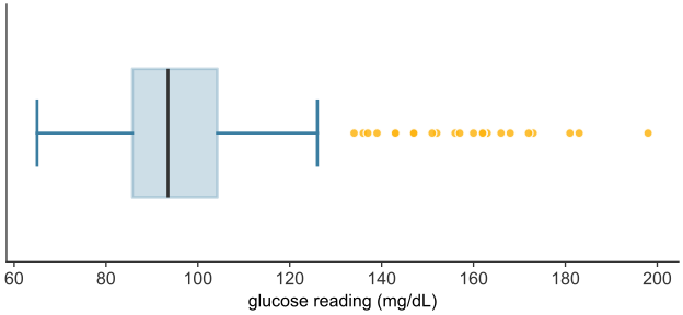
scripts/03_statistics/04_numerical_data/gen_numerical_data.py.
The histogram shows the right tail as a run of low bars. The box plot (see Figure 25.6) shows it as 25 points flagged beyond the upper whisker. A box plot gives five statistics: the lower whisker end, \(Q_1\), the median, \(Q_3\), and the upper whisker end. When points are flagged, the upper whisker end is the largest value that is not an outlier. The largest reading, \(198\) mg/dL, is therefore not shown.
The median and the IQR are the robust counterparts to the mean and the standard deviation. Neither moves much when a value in the tail is extreme, because both depend only on the middle half of the data. Reporting median (IQR) rather than mean (SD) is the usual choice when skew or outliers are expected.
Rescaling a summary: linear transformations
Data is sometimes recorded in one unit and needed in another: a temperature in Celsius reported in Fahrenheit, a concentration in \(\mu\text{g/mL}\) reported in \(\text{mg/L}\). Such a change is a linear transformation: a value \(x\) becomes \(y = ax + b\) for fixed constants \(a\) and \(b\). Its effect on a distribution’s center and spread follows directly from the definitions already in hand, without recomputing from the transformed values one at a time.
The mean transforms the way each value does, because the mean is a sum divided by the count, and scaling and shifting carry through that sum: \[\bar{y} = a\bar{x} + b.\] The spread, however, is not affected by the shift \(b\) at all: sliding the values by the same amount slides the mean by that amount too, leaving each deviation from the mean, and hence the spread, untouched. Scaling by \(a\) does change the spread, by the same factor \(a\) (taking \(|a|\), since a spread cannot be negative): \[s_y = |a|\,s_x, \qquad \mathrm{Var}(y) = a^2\,\mathrm{Var}(x).\] Variance scales by \(a^2\), not \(a\), because it is built from squared deviations. A shift changes where a distribution sits; only a scaling changes how spread out it is.
Populations and samples
The formulas so far have treated a set of values as though those values were all there is. In a trial they are not. The quantity a study cares about is a property of an entire population: all patients who might receive the treatment, not merely the hundred enrolled. What a study can measure is a sample, the subset actually observed. A population is the complete collection of individuals under study. Its summaries, the mean, variance, and standard deviation of the whole population, are called parameters and are written with Greek letters: the population mean \(\mu\), variance \(\sigma^2\), and standard deviation \(\sigma\). Parameters are fixed numbers, but they are almost always unknown, because the whole population cannot be measured.
A sample is a subset of the population, of size \(n\), actually measured. Its summaries, computed by the same arithmetic on the data in hand, are called statistics and are written with Latin letters: the sample mean \(\bar{x}\), variance \(s^2\), and standard deviation \(s\). A statistic is known, since it is computed from data, but variable, since a different sample would yield a different value. Inference uses a known, variable statistic to estimate an unknown, fixed parameter: it reasons from \(\bar{x}\) to \(\mu\).
| Quantity | Population parameter (fixed, unknown) | Sample statistic (computed, variable) |
|---|---|---|
| size | \(N\) | \(n\) |
| mean | \(\mu\) | \(\bar{x}\) |
| variance | \(\sigma^2\) | \(s^2\) |
| standard deviation | \(\sigma\) | \(s\) |
Each statistic on the right estimates the parameter on its left.
Estimating the variance: why \(n-1\)
The sample mean \(\bar{x}\) applies the mean’s formula to the sample and estimates \(\mu\). The sample variance needs one adjustment.
The population variance is the mean squared deviation about the population mean \(\mu\). In a sample, \(\mu\) is unknown, so the natural estimate replaces it with the sample mean \(\bar{x}\) and averages the squared deviations about that:
\[ \frac{1}{n}\sum_{i=1}^{n} (x_i - \bar{x})^2 . \]
This comes out systematically too small, and the reason is the least-squares property of the mean. Because \(\bar{x}\) is the value that minimizes the sum of squared deviations, \(\sum_i (x_i - \bar{x})^2\) is smaller than the sum about any other point, in particular smaller than \(\sum_i (x_i - \mu)^2\), the quantity the population variance is actually built from. Dividing the too-small numerator by \(n\) therefore underestimates \(\sigma^2\). A sample, forced to measure its spread about its own mean rather than the true one, tends to look a little less spread out than the population it came from.
The correction divides by \(n-1\) instead of \(n\):
\[ s^2 \;=\; \frac{1}{n-1}\sum_{i=1}^{n} (x_i - \bar{x})^2, \qquad s = \sqrt{s^2}. \]
The slightly smaller divisor inflates the estimate by just enough to compensate, on average, for the deficit. The adjustment is called Bessel’s correction, and \(n-1\) is the number of degrees of freedom of the estimate: the \(n\) deviations \(x_i - \bar{x}\) are bound by one exact relation, they sum to zero, so once any \(n-1\) of them are fixed, the last is determined, and only \(n-1\) are free to vary. The effect is clearest in a simulation on a population whose true variance is known because the population was constructed.
rng = np.random.default_rng(0)

# A model population of 100,000 six-month-old infant lengths (cm), simulated so
# that the true parameters mu, sigma are known exactly and estimates can be judged.
population = rng.normal(67.0, 2.5, size=100_000)
mu = population.mean()          # population parameters -- computable only because
sigma = population.std(ddof=0)  # the entire population happens to be in hand here
print(f"population parameters:   mu    = {mu:.2f} cm     sigma = {sigma:.2f} cm")

# One sample of 12 infants -- what a small study actually observes.
sample = rng.choice(population, size=12, replace=False)
print(f"one sample (n = 12):     x-bar = {sample.mean():.2f} cm     "
      f"s = {sample.std(ddof=1):.2f} cm")
population parameters: mu = 67.00 cm sigma = 2.50 cm
one sample (n = 12): x-bar = 66.32 cm s = 2.15 cmThe sample of twelve returns statistics close to, but not equal to, the parameters. A simulation isolates the divisor’s effect. For each sample size \(n\), it draws twenty thousand samples from the population, computes the variance of each both ways (dividing by \(n\) and by \(n-1\)), and averages. The average of an estimate over many samples reveals its systematic bias, if any.
sigma2 = population.var(ddof=0)      # the true population variance to be estimated
sizes = np.arange(2, 31)
R = 20_000                           # samples drawn at each sample size
avg_divN, avg_divN1 = [], []
for n in sizes:
    s = rng.choice(population, size=(R, n), replace=True)
    avg_divN.append(s.var(axis=1, ddof=0).mean())    # divide by n
    avg_divN1.append(s.var(axis=1, ddof=1).mean())   # divide by n - 1

fig, ax = plt.subplots()
ax.axhline(sigma2, color="black", lw=1.5, ls=":", label=r"true $\sigma^2$")
ax.plot(sizes, avg_divN,  "o-", color=GOLD, ms=4, label=r"estimate dividing by $n$")
ax.plot(sizes, avg_divN1, "o-", color=BLUE,   ms=4, label=r"estimate dividing by $n-1$")
ax.set_xlabel(r"sample size $n$")
ax.set_ylabel("average variance estimate\n(over 20,000 samples)")
ax.legend()
plt.show()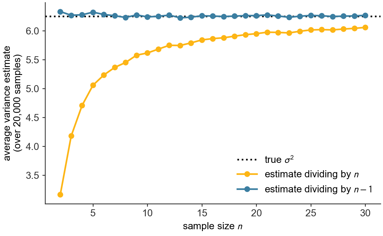
scripts/03_statistics/04_numerical_data/gen_numerical_data.py.
The estimate that divides by \(n-1\) hugs the true variance \(\sigma^2\) across the sample sizes shown (see Figure 25.7): it is, on average, exactly right. The estimate that divides by \(n\) sits below it, badly for the smallest samples and less so as \(n\) grows: at \(n=2\) it averages only half of \(\sigma^2\), at \(n=10\) about nine-tenths, at \(n=30\) within a few percent. The correction is largest in small samples, such as those of an early clinical trial, and shrinks toward zero in large datasets. This is why, unless a set of values genuinely is the whole population of interest, the sample variance and standard deviation, dividing by \(n-1\), are the ones to report.
The two conventions are a common source of silent error, because different tools default differently. In numpy, np.var and np.std divide by \(n\) by default (ddof=0, the population form); in pandas, a Series’ .var() and .std() divide by \(n-1\) by default (ddof=1, the sample form). Both accept a ddof argument to override the default. When a sample variance is intended, the usual case, set ddof=1. The code here states the divisor explicitly on every call so that nothing is left to a default.
The sampling distribution of a statistic is the pattern its value traces out over the many samples that might have been drawn. It shows how closely a sample statistic lands on its parameter, and how that improves as \(n\) grows. From this follow both the law that the sample mean converges on the population mean and the amount by which a sample of size \(n\) typically misses.
Comparing two distributions: overlaid histograms
Whether a treatment works is a question about two distributions. A trial measures an outcome across a treated group and a control group, and the treatment has an effect only if the treated group’s distribution differs from the control’s: shifted higher, or narrower, or otherwise moved. The most direct way to look for such a difference is to overlay the two distributions on a single pair of axes and compare their shapes by eye.
An overlay is legitimate only when the distributions are commensurable: the same variable, in the same units, binned the same way, on the same axes. The example uses a historical dataset. In the 1880s Francis Galton recorded the statures of many families to study inheritance (Galton 1886); a subset gives the heights, in inches, of \(179\) adult sons alongside their fathers (Adhikari et al. 2022). Father’s height and son’s height are the same variable measured on two groups, the same structure as a treated and a control group, so their distributions can be laid directly over each other.
heights = pd.read_csv(DATA + "sons_heights.csv")
print(f"fathers: mean {heights['father'].mean():.1f} in    "
      f"sons: mean {heights['son'].mean():.1f} in")

bins = np.arange(60, 82, 2)                       # common bins, common axis
fig, ax = plt.subplots()
ax.hist(heights["father"], bins=bins, density=True, alpha=0.55,
        color=BLUE,   edgecolor="white", label="fathers")
ax.hist(heights["son"],    bins=bins, density=True, alpha=0.55,
        color=GOLD, edgecolor="white", label="sons")
ax.set_xlabel("height (inches)")
ax.set_ylabel("proportion per inch (density)")
ax.legend(loc="upper left")
plt.show()
fathers: mean 69.1 in sons: mean 70.5 in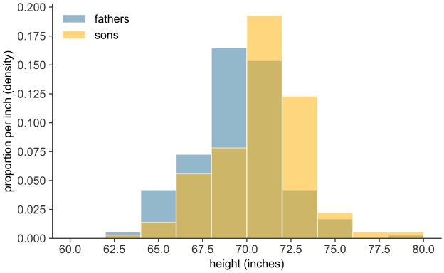
scripts/03_statistics/04_numerical_data/gen_numerical_data.py.
The two distributions have much the same breadth and the same rough symmetry, but the sons’ is displaced bodily to the right of the fathers’ by a little over an inch (see Figure 25.8). The printed means, \(69.1\) inches against \(70.5\), put a number on that shift. The sons, as a group, are taller. The density scale is used here even though the two groups are the same size: had they differed, raw counts would have made the larger group’s bars taller everywhere regardless of shape, corrupting the comparison. The overlay suggests a difference; it does not establish one. A visible shift in a sample this size might reflect a real difference between the underlying populations, or it might be a difference that two samples drawn from the same population produce by chance. The same ambiguity arises in the Dermagraft trial, at \(30.0\%\) against \(18.3\%\). The hypothesis test decides between those readings.
Relating two variables: the scatter plot
A question about two numerical variables, measured on the same individuals, is how they move together: whether, across meals, a larger carbohydrate load tends to accompany a higher glucose peak, or whether, across patients, a higher dose accompanies a faster recovery. The picture for a pair of numerical variables is the scatter plot: each individual becomes one point, its horizontal position the first variable and its vertical position the second.
rng = np.random.default_rng(33)
carbs = rng.uniform(20, 90, 40).round(0)
peak_glucose = (85 + 0.7 * carbs + rng.normal(0, 8, 40)).round(0)

fig, ax = plt.subplots()
ax.scatter(carbs, peak_glucose, color=BLUE, edgecolor="white", s=55, zorder=3)
ax.set_xlabel("carbohydrate in meal (g)")
ax.set_ylabel("peak glucose after meal (mg/dL)")
plt.show()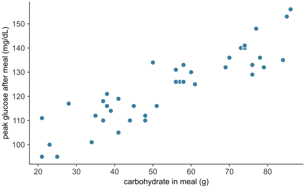
scripts/03_statistics/04_numerical_data/gen_numerical_data.py.
Each of the \(40\) points is one hypothetical meal, placed by its carbohydrate content and the peak glucose reading after it. The cloud slopes upward (see Figure 25.9): meals with more carbohydrate tend to be followed by higher peaks, a positive association between the two variables. (A downward slope would be a negative association; a shapeless cloud, no association.) The points scatter around the trend, so the association is not exact. In these data the scatter reflects the random variation in each meal’s response.
A scatter plot displays an association; it does not measure its strength or fit a line to it. Regression quantifies the relationship between two numerical variables.
From summaries to inference
A distribution is summarized by a center and a spread, each in a population form and a sample form. The Dermagraft trial’s question, does the treatment work, becomes a question about these summaries. Each arm is reduced to a mean outcome and a standard deviation, and the treatment has an effect only if the treated mean exceeds the control mean by more than chance alone, given the spread within the arms and the sample size, would produce. Deciding when a difference between two means is real rather than accidental requires knowing how much a sample mean would vary if the trial were repeated. The sampling distribution describes that variation.