30 Inference on Numerical Data
Many outcomes are numerical measurements: an ulcer’s area in \(\text{cm}^2\), or a wound’s healing time in days. The inference methods for a proportion (categorical data) carry over, with the sample mean \(\bar x\) in place of \(\hat p\). A null hypothesis \(H_0\) states that there is no difference or no effect. A p-value is the probability, computed under \(H_0\), of a result at least as extreme as the one observed.
import numpy as np
import matplotlib.pyplot as plt
from math import erf, sqrt, gamma, pi

BLUE, GOLD, GREEN, PURPLE = "#0072B2", "#E69F00", "#009E73", "#CC79A7"

def Phi(z):
    "Standard normal CDF, for contrast with the t-distribution below."
    return 0.5 * (1.0 + erf(z / sqrt(2.0)))

def two_sided_normal_p(z):
    return 2.0 * (1.0 - Phi(abs(z)))
Sampling distribution of the sample mean
Each sample gives a different \(\bar x\). The Central Limit Theorem describes their distribution.
Central Limit Theorem for the sample mean. When a sufficiently large sample of \(n\) independent observations is drawn from a population with mean \(\mu\) and standard deviation \(\sigma\), the sampling distribution of \(\bar x\) is nearly normal, with
\[ \text{Mean} = \mu, \qquad \text{Standard error (SE)} = \frac{\sigma}{\sqrt n}. \]
The standard error is the standard deviation of \(\bar x\) across repeated samples. It depends on \(\sigma\) and on \(n\).
If \(\sigma\) is known, the standardized statistic
\[ z = \frac{\bar x - \mu_0}{\sigma/\sqrt n} \]
is compared with the standard normal curve when testing \(H_0: \mu = \mu_0\). The p-value and the decision rule are the same as for the proportion tests.
Conditions for the sample mean
Two conditions are required to apply the Central Limit Theorem to \(\bar x\).
Independence. The observations must be independent. The most common way to satisfy this is a simple random sample from the population. Data from a random process, such as repeated rolls of a die, also satisfy the condition.
Normality. When the sample is small, the observations must come from a normally distributed population. The requirement relaxes as \(n\) grows.
To check normality, follow these steps (Diez et al. 2019):
- Plot the data as a histogram or a box plot. Note any outliers.
- If \(n < 30\) and there are no clear outliers, assume the data come from a nearly normal distribution.
- If \(n \geq 30\) and there are no particularly extreme outliers, assume the sampling distribution of \(\bar x\) is nearly normal, even if the observations are not.
- Ask whether the population could have moderate skew (\(n < 30\)) or particularly extreme outliers (\(n \geq 30\)). If so, the normal model does not apply.
A sample of \(n = 15\) with no clear outliers passes step 2. A sample of \(n = 50\) with one outlier about five times further from the center than the next furthest value fails step 3.
The t-distribution
In practice \(\sigma\) is rarely known, so the standard error cannot be computed directly. The sample standard deviation \(s\) takes its place:
\[ \mathrm{SE} = \frac{\sigma}{\sqrt n} \approx \frac{s}{\sqrt n}. \]
This works well when \(n\) is large and \(s\) is an accurate estimate of \(\sigma\). With a small sample, \(s\) is itself a noisy estimate, sometimes well below \(\sigma\) and sometimes well above it. Dividing by such an \(s\) produces occasional large values that the normal curve does not predict, so the standardized statistic has heavier tails than the normal.
When \(\sigma\) is estimated from a small sample of normal observations, the standardized statistic follows the \(t\)-distribution. It was published in \(1908\) by William Sealy Gosset (Student 1908), who worked at the Guinness brewery in Dublin and wrote under the pseudonym “Student.” The \(t\)-distribution is bell-shaped and centered at zero, like the normal, but its tails are thicker. Its single parameter is the degrees of freedom, \(\nu = n - 1\). As \(\nu\) grows, \(s\) becomes a more accurate estimate of \(\sigma\), and the \(t\)-distribution approaches the standard normal. When \(\nu\) is about 30 or more, the two are nearly indistinguishable.
The conditions for the \(t\)-model are the conditions for \(\bar x\) given above: independence, and the normality rules of thumb.
# Simulate the standardized statistic t = (x-bar - mu) / (s / sqrt(n)) for small
# samples drawn from a normal population, and compare its distribution to the
# standard normal. Because s is estimated from few points, t strays further than a
# z-score would -- this is the t-distribution's heavier tails, seen by simulation.
rng = np.random.default_rng(0)
mu_pop, sigma_pop, reps = 0.0, 1.0, 200_000

def t_statistics(n):
    samples = rng.normal(mu_pop, sigma_pop, size=(reps, n))
    xbar = samples.mean(axis=1)
    s = samples.std(axis=1, ddof=1)                   # sample SD (divide by n-1)
    return (xbar - mu_pop) / (s / np.sqrt(n))

grid = np.linspace(-6, 6, 1201)
normal_density = np.exp(-0.5 * grid**2) / np.sqrt(2 * np.pi)

fig, ax = plt.subplots(figsize=(7.5, 4.2))
for n, color in [(3, GOLD), (10, GREEN)]:
    ax.hist(t_statistics(n), bins=np.linspace(-6, 6, 121), density=True,
            histtype="step", lw=2, color=color,
            label=f"simulated t,  n = {n}  (ν = {n-1})")
ax.plot(grid, normal_density, color=BLUE, lw=2, label="standard normal N(0, 1)")
ax.set_xlabel("standardized statistic")
ax.set_ylabel("density")
ax.legend(fontsize=8)

# Quantify the excess mass in the tails: how often does |t| exceed 2?
print("chance the standardized statistic exceeds 2 in magnitude:")
for n in [3, 10, 30]:
    frac = (np.abs(t_statistics(n)) > 2).mean()
    print(f"  n = {n:>2} (ν = {n-1:>2}):  P(|t| > 2) = {frac*100:4.1f}%"
          f"      standard normal: 4.6%")
plt.show()
chance the standardized statistic exceeds 2 in magnitude:
n = 3 (ν = 2): P(|t| > 2) = 18.4% standard normal: 4.6%
n = 10 (ν = 9): P(|t| > 2) = 7.7% standard normal: 4.6%
n = 30 (ν = 29): P(|t| > 2) = 5.5% standard normal: 4.6%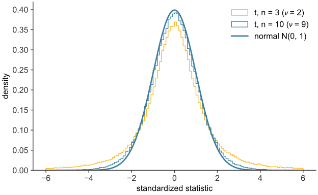
scripts/03_statistics/09_inference_numerical/gen_inference_numerical.py.
The heavier tails change the test (see Figure 30.1). A statistic must reach further from zero to be as surprising under the \(t\)-distribution as under the normal, so the same statistic gives a larger p-value. For one sample, the \(t\)-statistic has the form of the z-statistic with \(s\) in place of \(\sigma\):
\[ t = \frac{\bar x - \mu_0}{s/\sqrt n}, \qquad \nu = n - 1. \]
- z-test: use when \(\sigma\) is known. For a proportion, the variance \(p(1-p)\) is fixed by the rate itself, so the z-test of the categorical chapter applies directly, with no separate spread to estimate.
- t-test: use when comparing means and \(\sigma\) is unknown, which is the usual case. Compare the statistic with the \(t\)-distribution with \(\nu = n-1\) (one sample) or \(\nu = n_1 + n_2 - 2\) (two pooled samples). As \(\nu\) grows, the \(t\)-distribution approaches the normal, so the two tests agree for large samples.
One-sample t-interval and t-test
Confidence interval for a mean
A confidence interval for \(\mu\) has the form point estimate \(\pm\, t^\star \times \mathrm{SE}\). With \(\sigma\) unknown, the interval is
\[ \bar x \;\pm\; t^\star_{\nu} \cdot \frac{s}{\sqrt n}, \qquad \nu = n - 1, \]
where \(t^\star_\nu\) is the cutoff on the \(t\)-distribution with \(\nu\) degrees of freedom that leaves the chosen confidence level between \(-t^\star_\nu\) and \(t^\star_\nu\). It plays the role of \(z^\star\) for the normal interval.
To construct the interval:
- Prepare. Identify \(\bar x\), \(s\), \(n\), and the confidence level.
- Check. Verify independence and the normality rules of thumb.
- Calculate. Compute \(\mathrm{SE} = s/\sqrt n\), find \(t^\star\) for \(\nu = n - 1\), and compute \(\bar x \pm t^\star \cdot \mathrm{SE}\).
- Conclude. Interpret the interval in the context of the problem.
A \(95\%\) confidence interval gives a range of plausible values for \(\mu\). It does not describe the individual observations.
Consider the pilot’s device arm alone: eight ulcers with mean reduction \(\bar x = 3.83\ \text{cm}^2\) and sample standard deviation \(s = 1.04\ \text{cm}^2\). With \(n = 8\), \(\nu = 7\), and \(t^\star_7 = 2.365\) for \(95\%\) confidence,
xbar, s, n = 3.83, 1.04, 8
dof = n - 1
tstar = 2.365                          # t*, nu = 7, 95% confidence
se = s / np.sqrt(n)
moe = tstar * se

print(f"SE = {se:.3f} cm^2,   margin of error = {moe:.2f} cm^2")
print(f"95% CI = ({xbar - moe:.2f}, {xbar + moe:.2f}) cm^2")
SE = 0.368 cm^2, margin of error = 0.87 cm^2
95% CI = (2.96, 4.70) cm^2The device arm’s mean ulcer-area reduction is estimated at \(3.83\ \text{cm}^2\), and the \(95\%\) confidence interval runs from \(2.96\) to \(4.70\ \text{cm}^2\). The interval is wider than a large-sample interval with the same \(s\), because \(t^\star_7 = 2.365\) exceeds the normal value \(1.96\). The extra width reflects the uncertainty of estimating \(\sigma\) from eight ulcers.
Hypothesis test for a mean
The test of \(H_0: \mu = \mu_0\) follows the four steps of any hypothesis test:
- Prepare. State \(H_0\) and \(H_1\), the significance level \(\alpha\), and the values of \(\bar x\), \(s\), and \(n\).
- Check. Verify the independence and normality conditions.
- Calculate. Compute the standard error \(s/\sqrt n\), the t-statistic \(T = (\bar x - \mu_0)/\mathrm{SE}\), and its p-value on \(\nu = n-1\) degrees of freedom. The p-value is the area in the \(t\)-distribution beyond \(T\). For a two-sided alternative \(H_1: \mu \neq \mu_0\), double the area in one tail.
- Conclude. Reject \(H_0\) if the p-value is at most \(\alpha\). Otherwise fail to reject \(H_0\). Equivalently, reject \(H_0\) when \(|T|\) exceeds the critical value \(t^\star\), the cutoff that leaves \(\alpha/2\) of the \(t\)-distribution in each tail for a two-sided test. State the conclusion in the context of the problem.
A one-sided alternative, \(H_1: \mu > \mu_0\) or \(H_1: \mu < \mu_0\), uses the area in one tail only. It is justified only when the direction was fixed before the data were collected. Otherwise the two-sided test applies.
Paired data: before-and-after measurements on the same patients
Not every continuous comparison involves two separate groups. Many instead measure the same individual twice, once before an intervention and once after. Suppose ten patients each have their ulcer area measured at enrollment and again eight weeks later, on the device. Two sets of observations are paired when each observation in one set corresponds to exactly one observation in the other. Here each “after” value is matched to the “before” value from the same patient.
Analyzing the two columns as if they came from independent groups would discard information. Some patients start with larger ulcers than others, and that patient-to-patient variation has nothing to do with the treatment. Subtracting each patient’s own after-value from their own before-value removes it. The quantity analyzed is the difference,
\[ d_i = (\text{before})_i - (\text{after})_i, \]
one number per patient. The paired comparison then reduces to a one-sample \(t\)-test on the differences. The null hypothesis is that the mean difference is zero (no change), and the test statistic is
\[ t = \frac{\bar d - 0}{s_d/\sqrt n}, \qquad \nu = n - 1, \]
where \(\bar d\) and \(s_d\) are the mean and sample standard deviation of the \(n\) differences. The confidence interval for the mean difference is \(\bar d \pm t^\star_\nu\, s_d/\sqrt n\).
# Ten patients, ulcer area (cm^2) measured before treatment and again after 8 weeks
# on the device -- the same patients both times, so the two columns are paired.
before = np.array([5.2, 3.8, 6.1, 4.5, 7.0, 3.2, 5.8, 4.9, 6.4, 5.0])
after  = np.array([3.9, 3.0, 4.8, 3.6, 5.1, 2.9, 4.0, 3.5, 4.7, 3.8])
diffs = before - after                    # one difference per patient
n = diffs.size

mean_d = diffs.mean()
s_d = diffs.std(ddof=1)
se_d = s_d / np.sqrt(n)
t_stat = mean_d / se_d                    # H0: mean reduction = 0
dof = n - 1

print(f"mean reduction = {mean_d:.2f} cm^2,   s_d = {s_d:.2f} cm^2,   n = {n}")
print(f"SE = {se_d:.3f} cm^2,   t = {t_stat:.2f}   on nu = {dof}")
mean reduction = 1.26 cm^2, s_d = 0.49 cm^2, n = 10
SE = 0.156 cm^2, t = 8.09 on nu = 9def t_pdf(x, nu):
coef = gamma((nu + 1)/2) / (np.sqrt(nu*pi) * gamma(nu/2))
return coef * (1 + x**2/nu) ** (-(nu + 1)/2)
def t_one_sided_p(t_obs, nu):
xs = np.linspace(t_obs, t_obs + 60, 400_000)
return np.trapezoid(t_pdf(xs, nu), xs)
p_one = t_one_sided_p(t_stat, dof) # H1: mean reduction > 0 -- a one-sided test,
print(f"one-sided p-value = {p_one:.6f}") # legitimate here since a negative "reduction"
# (the ulcer growing) is not the question asked
fig, axes = plt.subplots(1, 2, figsize=(10, 4))
axes[0].hist(diffs, bins=np.arange(0, 2.2, 0.2), color=BLUE, edgecolor="white")
axes[0].axvline(mean_d, color=GOLD, lw=2, ls="--", label=f"mean reduction = {mean_d:.2f}")
axes[0].axvline(0, color="0.4", lw=1.5, ls=":", label="no change")
axes[0].set_xlabel("reduction in ulcer area, before − after (cm²)")
axes[0].set_ylabel("number of patients")
axes[0].legend(fontsize=8)
grid = np.linspace(-4, 10, 2001)
axes[1].plot(grid, t_pdf(grid, dof), color=BLUE, lw=2, label=f"t-distribution, ν = {dof}")
tail = grid >= t_stat
axes[1].fill_between(grid[tail], t_pdf(grid[tail], dof), color=GOLD, alpha=0.6,
label=f"one-sided p ≈ {p_one:.1e}")
axes[1].axvline(t_stat, color=GREEN, lw=2, label=f"observed t = {t_stat:.2f}")
axes[1].set_xlabel("t")
axes[1].set_ylabel("density")
axes[1].legend(fontsize=8, facecolor="white", edgecolor="none", framealpha=0.9) # opaque: the peak and the observed-t line both cross every open corner
plt.show()one-sided p-value = 0.000010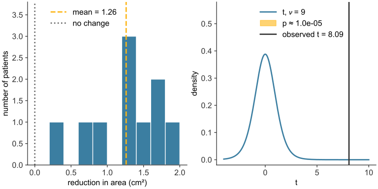
scripts/03_statistics/09_inference_numerical/gen_inference_numerical.py.
All ten ulcers shrank, by amounts from \(0.3\) to \(1.9\ \text{cm}^2\) (see Figure 30.2). The mean reduction is \(1.26\ \text{cm}^2\), with \(t = 8.09\) on \(\nu = 9\) degrees of freedom, and the one-sided p-value is about \(0.00001\). The \(95\%\) confidence interval for the mean reduction is \(1.26 \pm 2.262 \times 0.156\), or \((0.91,\ 1.61)\ \text{cm}^2\). Pairing removes the patient-to-patient variation, so the differences \(d_i\) are less spread out than the before or the after values alone. A paired design can therefore detect an effect with fewer patients than an unpaired design needs. The test is one-sided because the trial asks whether the device reduces ulcer area, a direction fixed before the data were collected. A two-sided test is the more conservative choice.
Comparing two independent groups
Difference of two means
When two groups are independent, the parameter is the difference \(\mu_1 - \mu_2\), and the point estimate is \(\bar x_1 - \bar x_2\). Two conditions must hold for the \(t\)-distribution to apply:
- Independence, extended. The observations are independent within each group and between the two groups, as in independent random samples or a randomized experiment.
- Normality. The outlier rules of thumb are checked for each group separately.
The standard error uses the sample standard deviations of the two groups:
\[ \mathrm{SE} = \sqrt{\frac{s_1^2}{n_1} + \frac{s_2^2}{n_2}}. \]
The test statistic is \(T = \dfrac{(\bar x_1 - \bar x_2) - 0}{\mathrm{SE}}\) under \(H_0: \mu_1 - \mu_2 = 0\). Software estimates the degrees of freedom from both groups’ variances (Welch’s approximation). Without software, use the smaller of \(n_1 - 1\) and \(n_2 - 1\), which gives a slightly conservative p-value. The confidence interval is \((\bar x_1 - \bar x_2) \pm t^\star \cdot \mathrm{SE}\).
Pool the standard deviations only when background research gives good reason to believe the two population standard deviations are nearly equal. The pooled estimate then uses both samples:
\[ s_p = \sqrt{\frac{(n_1 - 1)\,s_1^2 + (n_2 - 1)\,s_2^2}{n_1 + n_2 - 2}}, \]
\[ t = \frac{\bar x_1 - \bar x_2}{s_p\sqrt{\tfrac{1}{n_1} + \tfrac{1}{n_2}}}, \qquad \nu = n_1 + n_2 - 2. \]
Pilot comparison
A small pilot compares the two arms on the continuous outcome. Eight ulcers treated with the device and eight given standard care have their areas measured before and after twelve weeks. The outcome is the reduction in area, in \(\text{cm}^2\). The ulcers are assumed to be independent within and between the two arms. The treated values run from \(2.2\) to \(5.2\ \text{cm}^2\) and the control values from \(1.2\) to \(3.5\ \text{cm}^2\), with no clear outliers in either arm. The example assumes equal spread, so it uses the pooled method.
# A small continuous-outcome pilot: reduction in ulcer area (cm^2) after 12 weeks.
treated = np.array([3.1, 4.5, 2.8, 5.2, 3.9, 4.1, 2.2, 4.8])   # device
control = np.array([1.9, 2.4, 3.0, 1.2, 2.8, 3.5, 1.7, 2.1])   # standard care
n1, n2 = treated.size, control.size

m1, m2 = treated.mean(), control.mean()
s1, s2 = treated.std(ddof=1), control.std(ddof=1)              # sample SDs (n-1)

sp = np.sqrt(((n1 - 1)*s1**2 + (n2 - 1)*s2**2) / (n1 + n2 - 2))  # pooled SD
se = sp * np.sqrt(1/n1 + 1/n2)                                   # SE of the difference
t_stat = (m1 - m2) / se
dof = n1 + n2 - 2

print(f"treated: mean = {m1:.2f} cm^2,   s = {s1:.2f},   n = {n1}")
print(f"control: mean = {m2:.2f} cm^2,   s = {s2:.2f},   n = {n2}")
print(f"pooled SD s_p = {sp:.2f} cm^2,   SE of difference = {se:.2f} cm^2")
print(f"t = {t_stat:.2f}   on nu = {dof} degrees of freedom")
treated: mean = 3.83 cm^2, s = 1.04, n = 8
control: mean = 2.33 cm^2, s = 0.75, n = 8
pooled SD s_p = 0.91 cm^2, SE of difference = 0.45 cm^2
t = 3.30 on nu = 14 degrees of freedom# The t-distribution's density (built from math.gamma), integrated in its tails to
# get the p-value -- the same "probability is area under the curve" rule the sampling
# section used for the normal, now applied to the heavier-tailed t.
def t_pdf(x, nu):
coef = gamma((nu + 1)/2) / (np.sqrt(nu*pi) * gamma(nu/2))
return coef * (1 + x**2/nu) ** (-(nu + 1)/2)
def t_two_sided_p(t_obs, nu):
xs = np.linspace(abs(t_obs), abs(t_obs) + 60, 400_000) # the far upper tail
tail = np.trapezoid(t_pdf(xs, nu), xs)
return 2 * tail # both tails, by symmetry
p_t = t_two_sided_p(t_stat, dof)
p_if_normal = two_sided_normal_p(t_stat)
print(f"two-sided p-value (t, nu = {dof}) = {p_t:.4f}")
print(f"for contrast, the same statistic read off the normal = {p_if_normal:.4f}")
# The observed t against its reference curve, with the p-value shaded in the tails.
grid = np.linspace(-5, 5, 2001)
fig, ax = plt.subplots(figsize=(7.5, 4))
ax.plot(grid, t_pdf(grid, dof), color=BLUE, lw=2, label=f"t-distribution, ν = {dof}")
ax.plot(grid, np.exp(-0.5*grid**2)/np.sqrt(2*pi), color="0.6", lw=1.5, ls="--",
label="standard normal")
tail_r, tail_l = grid >= t_stat, grid <= -t_stat
ax.fill_between(grid[tail_r], t_pdf(grid[tail_r], dof), color=GOLD, alpha=0.6)
ax.fill_between(grid[tail_l], t_pdf(grid[tail_l], dof), color=GOLD, alpha=0.6)
ax.axvline(t_stat, color=GREEN, lw=2, label=f"observed t = {t_stat:.2f}")
ax.axvline(-t_stat, color=GREEN, lw=1.2, ls="--")
ax.set_xlabel("t")
ax.set_ylabel("density")
ax.legend(fontsize=8)
plt.show()two-sided p-value (t, nu = 14) = 0.0052
for contrast, the same statistic read off the normal = 0.0010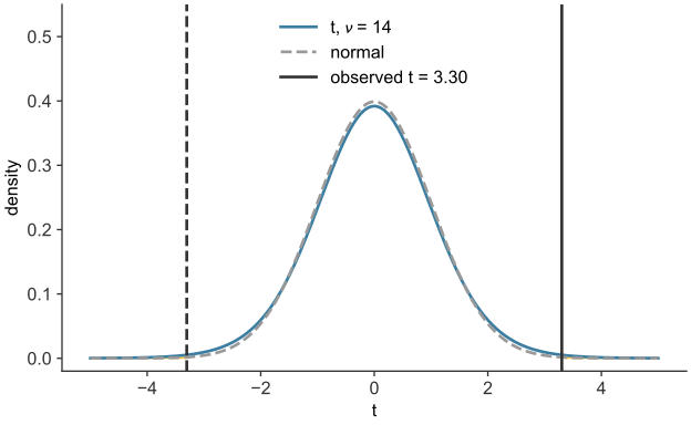
scripts/03_statistics/09_inference_numerical/gen_inference_numerical.py.
The device reduced ulcer area by \(3.83\ \text{cm}^2\) on average, against \(2.33\ \text{cm}^2\) for the control, a difference of \(1.50\ \text{cm}^2\). The \(t\)-statistic is \(3.30\) on \(\nu = 14\) degrees of freedom, so the two-sided p-value is \(p \approx 0.005\). At \(\alpha = 0.05\), reject \(H_0\): the difference is statistically significant. The \(95\%\) confidence interval for the difference is \(1.50 \pm 2.145 \times 0.454\), or \((0.53,\ 2.47)\ \text{cm}^2\).
Read off the normal curve, the same statistic gives \(p \approx 0.001\), about five times smaller than the \(t\)-based value. The two curves are similar near the center, but the \(t\)-distribution is lower at the peak and places more area in the tails, where the p-value is read (see Figure 30.3). Without the equal-spread assumption, the unpooled standard error is \(\sqrt{1.04^2/8 + 0.75^2/8} = 0.45\ \text{cm}^2\), with \(\nu = 7\), which gives \(t = 3.30\) and \(p \approx 0.013\). The conclusion at \(\alpha = 0.05\) is the same.
Power for a difference of means
A test’s power is the probability that it rejects \(H_0\) when a real effect exists. It equals one minus the probability of a Type II error (failing to reject \(H_0\) when the difference is real). A study with low power is called underpowered: a real effect of the planned size is likely to be missed. Power increases with the sample size, because a larger sample narrows the sampling distributions and pulls the null and alternative curves apart. For a difference of two means, the required sample size can be computed before any patient is enrolled.
Suppose a follow-up trial aims to detect a mean ulcer-area-reduction difference of \(\Delta = 1.0\ \text{cm}^2\) between two arms, and uses the pilot’s pooled standard deviation, \(\sigma \approx 0.91\ \text{cm}^2\), as a planning estimate. For a two-sided test at \(\alpha = 0.05\) with \(80\%\) power, the standard error of the difference must satisfy \(2.8 \times \mathrm{SE} \approx \Delta\). The constant \(2.8 = 1.96 + 0.84\). The \(1.96\) places the rejection boundary at \(\alpha = 0.05\). The \(0.84\) is the distance from that boundary to the alternative’s center, which leaves \(80\%\) of the alternative distribution beyond the boundary. With \(\mathrm{SE} = \sigma\sqrt{2/n}\) for two equal-sized arms, solving for \(n\) gives
\[ n \;=\; \frac{2\,(2.8)^2\,\sigma^2}{\Delta^2}. \]
sigma_planning = 0.91          # cm^2, from the pilot's pooled SD
for delta in [1.0, 0.5]:
    n_per_arm = 2 * (2.8**2) * sigma_planning**2 / delta**2
    print(f"to detect Delta = {delta} cm^2 at 80% power, alpha=0.05: "
          f"n = {n_per_arm:.1f} -> {int(np.ceil(n_per_arm))} patients per arm")
to detect Delta = 1.0 cm^2 at 80% power, alpha=0.05: n = 13.0 -> 13 patients per arm
to detect Delta = 0.5 cm^2 at 80% power, alpha=0.05: n = 51.9 -> 52 patients per armDetecting the full \(1.0\ \text{cm}^2\) effect needs about \(13\) patients per arm, because that effect is large relative to the pilot’s spread. Halving the effect to \(0.5\ \text{cm}^2\) quadruples the required sample to about \(52\) per arm. Because the standard error falls as \(1/\sqrt n\) (sampling distribution), resolving an effect half the size needs half the standard error, which takes four times the data.
Verdict on the device
For a continuous outcome, the question is how much the device reduced ulcer area. The \(16\)-patient pilot gave a mean difference of \(1.50\ \text{cm}^2\) between the device and control arms, with \(t = 3.30\) on \(14\) degrees of freedom and \(p \approx 0.005\). The ten paired patients showed a mean reduction of \(1.26\ \text{cm}^2\), and all ten ulcers shrank. Both analyses use the same four elements as the categorical case: a statistic, a standard error, a reference distribution, and a p-value. The \(t\)-distribution accounts for one difference: the spread of a continuous measurement is unknown and must be estimated from the data.
A p-value supports a conclusion only when the trial was designed well. Randomization, blinding, and a sample size chosen for the target effect and power are needed. A small p-value from a poorly designed study does not establish a cause.