17 Fick’s 1st Law
A drop of dye placed in a still glass of water spreads slowly outward, coloring the whole glass after many hours; this is diffusion. No bulk movement of fluid is required. Consider the case where a high number of molecules is confined to one side of a box. When the divider is removed, the molecules move by random motion to the other side (Figure 17.1). There is a flux due to diffusion.
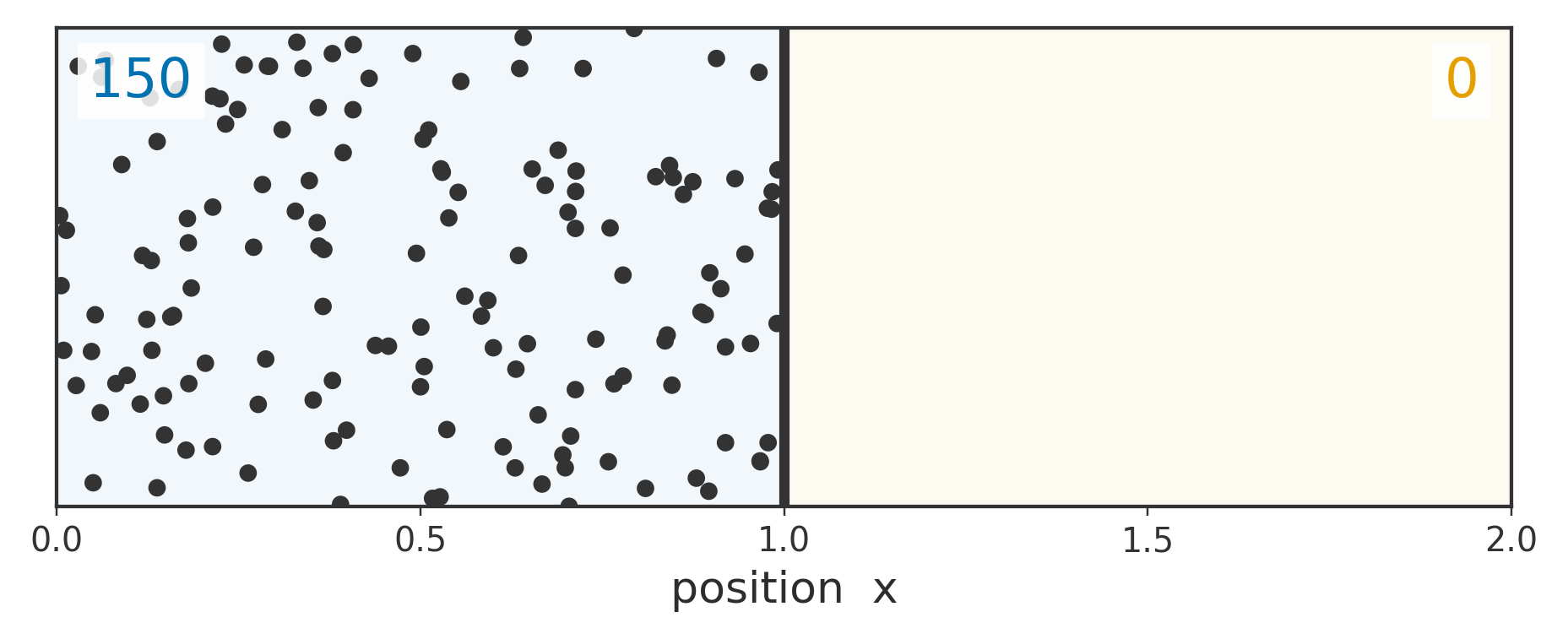
images/02_tissue/Diffusion/diffusion_partition.py.
Molecules cross the midline in both directions, but more cross to the right (Figure 17.2). Equilibrium occurs when the number of molecules is equal on both sides. However, the molecules are still moving, and, at any given instant, by random chance there may be a small imbalance.
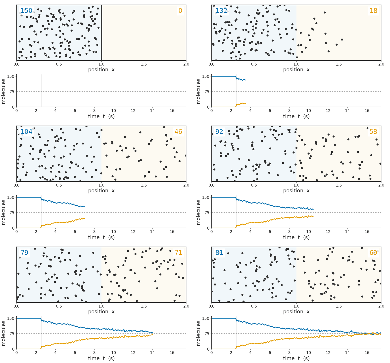
images/02_tissue/Diffusion/diffusion_partition.py.
Plot the concentration against \(x\), then its slope, then the flux, and the relationship becomes visible (Figure 17.3). The flux panel is the slope panel flipped over and rescaled, and nothing else: wherever the concentration falls steeply the flux is large, where the concentration flattens the flux dies away, and when the slope reaches zero so does the flux.
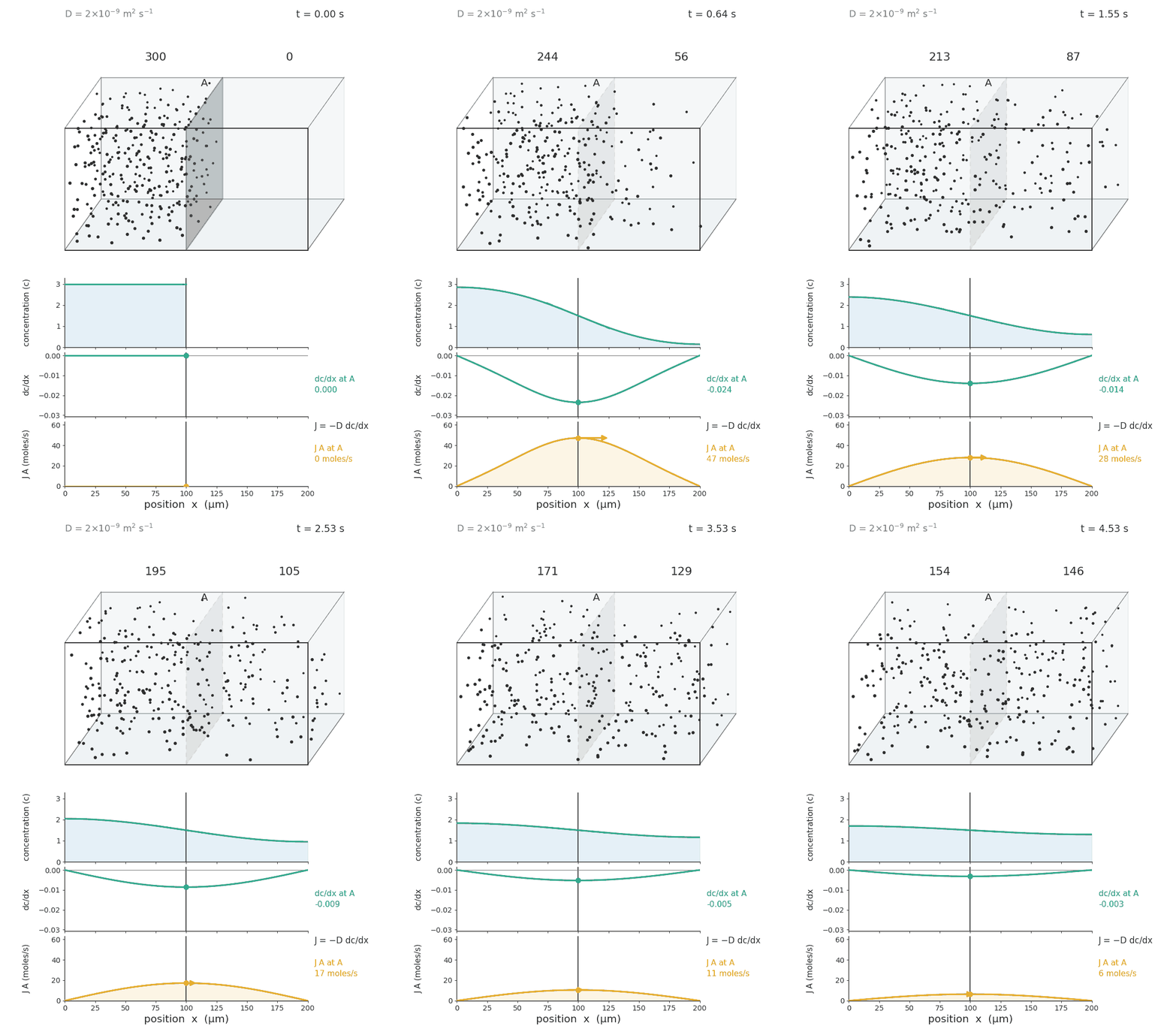
images/02_tissue/Diffusion/diffusion_gradient_3d.py.
Flux
Mass transport defined the flux as the amount of a species crossing unit area per unit time. Over a finite area and interval that is
\[J = \frac{n}{A\,t},\]
so \(n = JAt\) gives the amount delivered once the flux and the exposed area are known. Flux is a rate density, not a rate: doubling the area doubles the moles delivered each second but leaves \(J\) unchanged, which is what makes it a property of the transport rather than of the particular device it is measured in.
Fick’s First Law
The movie above depicts Fick’s law. When the concentration \(c(x)\) changes steeply, \(\mathrm{d}c/\mathrm{d}x\) is large, and so is the flux through a plane of area \(A\).
The minus sign is a convention with physical content. A species moves from where it is abundant toward where it is scarce, so wherever the concentration falls as \(x\) increases the gradient \(\partial c/\partial x\) is negative and \(J\) comes out positive, meaning transport in the \(+x\) direction. Flux and gradient always point in opposite directions.
Units and the diffusion coefficient
\(D\) is the diffusion constant. It is a measure of how quickly molecules diffuse through a medium and it varies with the properties of the medium, the diffusing species, and the temperature. What are its units?
The flux \(J\) has units of \(\text{mol m}^{-2}\text{s}^{-1}\). The concentration gradient \(\partial c/\partial x\) has units of \((\text{mol m}^{-3})/\text{m} = \text{mol m}^{-4}\). Therefore
\[[D] = \frac{[J]}{[\partial c/\partial x]} = \frac{\text{mol m}^{-2}\text{s}^{-1}}{\text{mol m}^{-4}} = \text{m}^2\text{s}^{-1}.\]
This is consistent with the microscopic definition \(D = (\Delta x)^2/(2\Delta t)\) derived from the random walk.
Where does Fick’s law come from?
Fick’s law is stated above as an empirical relation: flux is proportional to the gradient, with \(D\) the constant of proportionality. It can also be obtained by counting, from nothing more than the assumption that a molecule is equally likely to move one way as the other. This is similar to the random-walk derivation in the previous section.
Place a plane of area \(A\) at position \(x\), with a box of width \(\Delta x\) on each side (Figure 17.4). Let \(N_x\) be the number of molecules in the left box and \(N_{x+\Delta x}\) the number in the right.
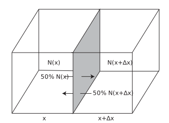
Write the counts as concentrations. Each box has volume \(A\,\Delta x\), so the concentration in it is the number of molecules divided by that volume,
\[c(x) = \frac{N_x}{A\,\Delta x}, \qquad\text{so}\qquad N_x = c(x)\,A\,\Delta x .\]
Let half of each box cross. Assume every molecule has an equal chance of staying on its own side or moving to the other side during a time \(\Delta t\). Then half the molecules in the left box cross to the right, and half of those in the right box cross to the left, so the net number crossing the plane is \(N_x/2 - N_{x+\Delta x}/2\).
Divide by area and time. Flux is the amount crossing unit area per unit time:
\[J(x,t) = \frac{\dfrac{N_x}{2} - \dfrac{N_{x+\Delta x}}{2}}{A\,\Delta t} .\]
Substitute the concentrations. Replacing each \(N\) with \(c\,A\,\Delta x\), the area cancels:
\[J(x,t) = \frac{1}{A} \left(\frac{c(x)\,A\,\Delta x - c(x + \Delta x)\,A\,\Delta x}{2\,\Delta t}\right) = \frac{\Delta x^2}{2\,\Delta t} \left(\frac{c(x) - c(x + \Delta x)}{\Delta x}\right) .\]
Take the limit. Writing the difference in the usual order, \(c(x + \Delta x) - c(x)\), introduces a minus sign, and as \(\Delta x \to 0\) the quotient becomes a derivative:
\[J = -\,\frac{\Delta x^2}{2\,\Delta t} \lim_{\Delta x \to 0}\left(\frac{c(x + \Delta x) - c(x)}{\Delta x}\right) = -\,\frac{\Delta x^2}{2\,\Delta t}\,\frac{\mathrm{d}c}{\mathrm{d}x} .\]
The group in front is a constant with units of \(\mathrm{m^2\,s^{-1}}\), which is the diffusion coefficient. Writing it as \(D\) gives Fick’s first law,
\[\boxed{\; J = -D\,\frac{\mathrm{d}c}{\mathrm{d}x} \;}\]
with
\[D = \frac{\Delta x^2}{2\,\Delta t},\]
the same combination of step size and step time the random walk produced from \(\langle x^2\rangle = 2Dt\).