27  The Binomial and Normal Distributions

Bernoulli trials and the binomial distribution

A single patient’s ulcer either heals within the trial’s follow-up window or it does not. Coded \(1\) for healed and \(0\) otherwise, this is a Bernoulli trial: one outcome with a fixed probability \(p\) of success (the binary variable coding). Treat \(n\) patients this way, each an independent Bernoulli trial with the same success probability \(p\), and count the total number of successes. That count is a binomial random variable.

NoteDefinition — random variable

A random variable is a numerical quantity whose value is determined by a random process. Before the process runs, its value is unknown. Its distribution lists each possible value and how likely it is. For a single Bernoulli trial, \(X = 1\) with probability \(p\) and \(X = 0\) otherwise. Once the process runs, \(X\) takes one value, which is the observation.

NoteDefinition — binomial random variable

A random variable \(X\) counts the number of successes in \(n\) independent Bernoulli trials, each with success probability \(p\). \(X\) is a binomial random variable, and its distribution is written \(\mathrm{Binomial}(n, p)\).

To find the probability of \(k\) successes, count the number of ways \(k\) successes can be arranged among the \(n\) trials, then multiply by the probability of one such arrangement. A single arrangement with \(k\) successes and \(n-k\) failures, in a particular order, has probability \(p^k(1-p)^{n-k}\) by the multiplication rule for independent events. The number of orders in which \(k\) successes can land among \(n\) trials is the binomial coefficient

\[ \binom{n}{k} = \frac{n!}{k!\,(n-k)!}, \]

read “\(n\) choose \(k\).”

NoteDerivation — the binomial probability formula

\[ P(X = k) \;=\; \binom{n}{k}\, p^k (1-p)^{n-k}, \qquad k = 0, 1, \ldots, n. \]

Four conditions must hold for this formula to apply: the trials are independent, their number \(n\) is fixed in advance, each trial is a clear success or failure, and the success probability \(p\) is the same on every trial. A clinical trial’s patients can approximately satisfy all four if they are enrolled independently and are assumed to share one healing probability under a treatment.

Flipping a coin ten times

Flip a fair coin \(10\) times and count the heads. Each flip is a trial with \(p(H) = 0.5\), so the count \(X\) is \(\mathrm{Binomial}(10,\ 0.5)\) (see Figure 27.1). The probability of exactly \(5\) heads is \(\binom{10}{5}/2^{10} = 252/1024 \approx 0.246\). The probability of at most \(2\) heads is \((1 + 10 + 45)/1024 = 56/1024 \approx 0.055\).

from math import comb

n = 10
probs = [comb(n, k) / 2**n for k in range(n + 1)]
print(f"P(5 heads) = {probs[5]:.3f}   P(X <= 2) = {sum(probs[:3]):.3f}")

P(5 heads) = 0.246   P(X <= 2) = 0.055

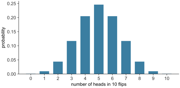
Figure 27.1: Probability of each number of heads in \(10\) flips of a fair coin, \(\mathrm{Binomial}(10,\ 0.5)\), from \(0\) to \(10\). The bars peak at \(5\) heads. Generated by scripts/03_statistics/06_binomial_and_normal/gen_binomial_and_normal.py.

Changing the coin changes the distribution (see Figure 27.2). The two are mirror images: a coin that lands heads \(80\%\) of the time gives heads counts that peak at \(8\), where the \(p(H) = 0.2\) coin peaks at \(2\).

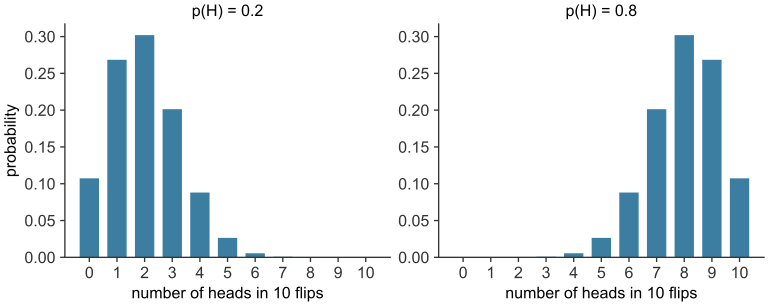
Figure 27.2: Number of heads in \(10\) flips for a coin with \(p(H) = 0.2\) (left) and \(p(H) = 0.8\) (right). The distributions are mirror images. Generated by scripts/03_statistics/06_binomial_and_normal/gen_binomial_and_normal.py.

The mean and variance of a binomial count

The mean and variance of a binomial random variable follow from the \(0\)/\(1\) mean and variance. Write \(X = Y_1 + \cdots + Y_n\), where \(Y_i\) is \(1\) if trial \(i\) succeeds and \(0\) otherwise. Each \(Y_i\) has mean \(p\) and variance \(p(1-p)\). Summing \(n\) of them adds the means. Independence lets the variances add as well.

\[ \mu_X = np, \qquad \sigma_X^2 = np(1-p), \qquad \sigma_X = \sqrt{np(1-p)}. \]

NoteDerivation — mean and variance of a binomial count

Each trial is a success with probability \(p\). Its mean is \(p\). Its squared distance from that mean is \((1-p)^2\) on a success and \(p^2\) on a failure, so its variance is

\[ p(1-p)^2 + (1-p)p^2 = p(1-p). \]

The count \(X\) is \(n\) trials added together. Their means add to \(np\). Because the trials are independent, they do not move together, so their variances add with no cross terms:

\[ \mathrm{Var}(X) = n\,p(1-p). \]

The device arm has a mean of \(39\) healed ulcers out of \(130\), with standard deviation about \(5.2\). The control arm has a mean of \(21\) out of \(115\), with standard deviation about \(4.1\). Dividing the standard deviation of the count by \(n\) gives the standard deviation of the healing rate: \(\sqrt{np(1-p)}/n = \sqrt{p(1-p)/n}\). This is the standard-error formula for a rate.

ImportantKnowledge check

A screening test correctly flags a diseased sample with probability \(p = 0.95\), independently across \(20\) diseased samples. Let \(X\) be the number correctly flagged. Identify \(n\), \(p\), and \(k\) for the event “exactly \(18\) flagged,” and give the mean and variance of \(X\).

NoteAnswer

Here \(n = 20\), \(p = 0.95\), and the event of interest is \(k = 18\), so \(P(X=18) = \binom{20}{18}(0.95)^{18}(0.05)^{2}\). The mean is \(\mu_X = np = 20 \times 0.95 = 19\), and the variance is \(\sigma_X^2 = np(1-p) = 20 \times 0.95 \times 0.05 = 0.95\).

The Normal distribution

The normal distribution (also called the Gaussian distribution) is a symmetric, bell-shaped model for a continuous measurement. It is fixed by two parameters: the mean \(\mu\), which sets the center, and the standard deviation \(\sigma\), which sets the spread.

NoteDerivation — the normal density from \(e^{-x^2}\)

Start from the bell-shaped function \(g(x) = e^{-x^2}\). It is positive, symmetric about \(0\), and peaks at \(1\). Four steps turn it into the normal density.

Step 1: the Gaussian integral. Let \(I = \int_{-\infty}^{\infty} e^{-x^2}\,dx\). Then

\[ I^2 = \int_{-\infty}^{\infty}\!\int_{-\infty}^{\infty} e^{-(x^2+y^2)}\,dx\,dy. \]

Switch to polar coordinates, \(x = r\cos\theta\), \(y = r\sin\theta\), with \(dx\,dy = r\,dr\,d\theta\):

\[ I^2 = \int_0^{2\pi}\!\!\int_0^{\infty} e^{-r^2}\,r\,dr\,d\theta = 2\pi \cdot \tfrac{1}{2} = \pi, \]

so \(I = \sqrt{\pi}\).

Step 2: make it a density. The area under \(g\) is \(\sqrt{\pi}\), so dividing by \(\sqrt{\pi}\) gives total area \(1\):

\[ f_1(x) = \frac{1}{\sqrt{\pi}}\, e^{-x^2}. \]

Step 3: shift to mean \(\mu\). Replace \(x\) with \(x - \mu\). The curve moves to be centered at \(\mu\), and the area is unchanged, because substituting \(u = x - \mu\) leaves \(\int f_1(u)\,du = 1\).

Step 4: scale to standard deviation \(\sigma\). Replace the exponent \((x-\mu)^2\) with \((x-\mu)^2/(2\sigma^2)\), which stretches the curve by \(\sigma\sqrt{2}\) horizontally. Substitute \(u = (x-\mu)/\sigma\), so \(dx = \sigma\,du\), and use \(\int_{-\infty}^{\infty} e^{-u^2/2}\,du = \sqrt{2\pi}\) (substitute \(u = \sqrt{2}\,v\) and apply Step 1). The area of the stretched curve is

\[ \int e^{-\frac{(x-\mu)^2}{2\sigma^2}}\,dx = \sigma\sqrt{2\pi}. \]

To keep the area at \(1\), the constant must be \(1/(\sigma\sqrt{2\pi})\):

\[ f(x) = \frac{1}{\sigma\sqrt{2\pi}}\, e^{-\frac{1}{2}\left(\frac{x-\mu}{\sigma}\right)^2}. \]

The shift sets the center and the scaling sets the width. The constant keeps the area at \(1\).

The model is specified by its density,

\[ f(x) = \frac{1}{\sigma\sqrt{2\pi}}\, e^{-\frac{1}{2}\left(\frac{x-\mu}{\sigma}\right)^2}, \]

where \(x\) is a value of the measurement, \(e \approx 2.718\) is Euler’s number, \(\mu\) is the mean (the center of the distribution), and \(\sigma\) is the standard deviation (the spread). The exponent equals zero at \(x = \mu\) and becomes more negative as \(x\) moves away from \(\mu\) in either direction. The density is therefore highest at the mean and falls off symmetrically on both sides.

The height \(f(x)\) is not a probability. It shows how densely measurements concentrate near \(x\). The normal distribution is a probability density function (PDF): its height is never negative, and its total area is \(1\). A PDF gives probabilities by integration. The probability that \(X\) falls between \(a\) and \(b\) is the integral of the density over that range:

\[ P(a \le X \le b) = \int_a^b f(x)\,dx. \]

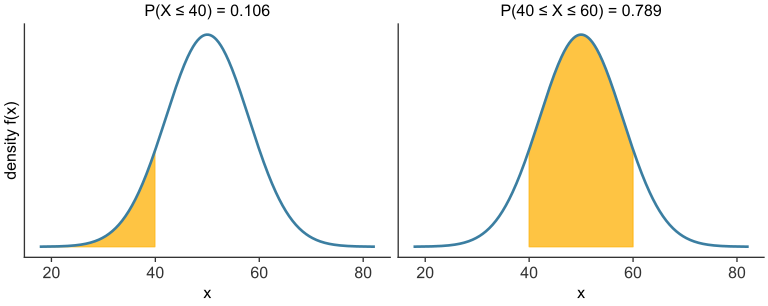
Figure 27.3: The normal density \(N(50,\ 8)\) with the integral shaded: the area to the left of \(40\) (left), and the area between \(40\) and \(60\) (right). Each shaded area is the probability in the title. Generated by scripts/03_statistics/06_binomial_and_normal/gen_binomial_and_normal.py.

Cutting the curve at \(40\) and at \(60\) gives the two shaded areas in Figure 27.3. Integrating from the far left up to \(40\) gives a tail probability.

The cumulative distribution function

The cumulative distribution function (CDF) of \(X\) is \(F(x) = P(X \le x)\), the area under the density to the left of \(x\). For the normal model, \(F(x) = \int_{-\infty}^{x} f(t)\,dt\). The standard normal CDF is written \(\Phi\), so \(\Phi(z) = P(Z \le z)\).

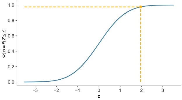
Figure 27.4: The standard normal CDF, \(\Phi(z) = P(Z \le z)\). The dashed lines mark \(z = 1.96\), where \(\Phi = 0.975\). Generated by scripts/03_statistics/06_binomial_and_normal/gen_binomial_and_normal.py.

Figure 27.4 plots \(\Phi\). It rises from \(0\) to \(1\). At \(z = 1.96\), \(\Phi(1.96) = 0.975\), so \(97.5\%\) of the area lies to the left.

Tail areas follow from \(\Phi\). The area to the right of \(z\) is \(1 - \Phi(z)\). The two-sided area beyond \(|z|\) is \(2\,(1 - \Phi(|z|))\), which is the p-value of a z-test (hypothesis test). The CDF also runs in reverse: \(\Phi(z) = 0.03\) gives \(z \approx -1.88\).

The mean and standard deviation define the curve (see Figure 27.5). The two curves have the same shape and width, but the second peak sits \(8\) units further right: changing \(\mu\) shifts the curve without changing its shape. On the right, \(N(50, 8)\) is compared with \(N(50, 4)\). Both peak at \(50\), but the second is narrower and taller, with peak height \(1/(4\sqrt{2\pi}) \approx 0.100\) against \(1/(8\sqrt{2\pi}) \approx 0.050\) for the first. Each curve encloses area \(1\), so a narrower curve must be taller. Changing \(\sigma\) stretches or compresses the curve around its center.

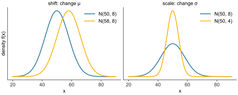
Figure 27.5: Left: \(N(50, 8)\) and \(N(58, 8)\), the same shape shifted by \(8\). Right: \(N(50, 8)\) and \(N(50, 4)\), the same center with a narrower, taller curve. Generated by scripts/03_statistics/06_binomial_and_normal/gen_binomial_and_normal.py.

Move the sliders in Figure 27.6. The curve is the density \(f(x)\) of \(N(\mu, \sigma)\). The readout gives the peak height, which falls as \(\sigma\) grows, and two probabilities. The area within one standard deviation of the mean is about \(0.683\) for every choice of the sliders.

viewof mu1 = Inputs.range([30, 70], {value: 50, step: 0.5, label: "mean μ"})
viewof sg1 = Inputs.range([2, 15], {value: 8, step: 0.5, label: "standard deviation σ"})

erf = (x) => {
  const s = Math.sign(x), a = Math.abs(x);
  const t = 1 / (1 + 0.3275911 * a);
  const y = 1 - (((((1.061405429 * t - 1.453152027) * t) + 1.421413741) * t - 0.284496736) * t + 0.254829592) * t * Math.exp(-a * a);
  return s * y;
}
Phi = (z) => 0.5 * (1 + erf(z / Math.sqrt(2)))

Plot.plot({
  width: 720,
  height: 340,
  marginLeft: 60,
  marginBottom: 55,
  x: {domain: [0, 100], label: "x", grid: true},
  y: {domain: [0, 0.5], label: "density f(x)", grid: true},
  marks: [
    Plot.line(d3.range(0, 100.01, 0.25).map(x => ({x, f: Math.exp(-0.5 * ((x - mu1) / sg1) ** 2) / (sg1 * Math.sqrt(2 * Math.PI))})),
      {x: "x", y: "f", stroke: "#3B7EA1", strokeWidth: 2.8}),
    Plot.ruleX([mu1], {stroke: "#D55E00", strokeDasharray: "4,3"})
  ]
})

Figure 27.6: Density of \(N(\mu, \sigma)\) for the sliders’ values. The peak height is \(1/(\sigma\sqrt{2\pi})\). Within one standard deviation of the mean the area is \(0.683\) for every choice of \(\mu\) and \(\sigma\).

html`<p>peak height $f(\mu) = ${(1 / (sg1 * Math.sqrt(2 * Math.PI))).toFixed(4)}$ &nbsp;·&nbsp; P(X ≤ ${(mu1 + 1 * sg1).toFixed(1)}) = ${Phi(1).toFixed(3)} &nbsp;·&nbsp; P(μ − σ ≤ X ≤ μ + σ) = ${(Phi(1) - Phi(-1)).toFixed(3)}</p>`

A normal distribution with mean \(\mu\) and standard deviation \(\sigma\) is written \(N(\mu, \sigma)\). The case \(\mu = 0\), \(\sigma = 1\) is the standard normal distribution, \(N(0, 1)\) (Diez et al. 2019).

Standard Normal Distribution

Every normal distribution has its own mean and standard deviation, so a table of normal areas would need a separate entry for each pair. The standard normal distribution, \(N(0, 1)\), removes that need. Any normal variable \(X\) can be converted to a standard normal variable \(Z\) by subtracting its mean and dividing by its standard deviation. Probabilities about \(X\) then become probabilities about \(Z\), and one table can be used for every case.

Measurements in different units and with different spreads become comparable once they are standardized.

NoteDerivation — converting any normal distribution to the standard normal

Let \(X \sim N(\mu, \sigma)\), with density \(f_X(x) = \frac{1}{\sigma\sqrt{2\pi}}\,e^{-(x-\mu)^2/(2\sigma^2)}\). We want a density for \(Z = (X - \mu)/\sigma\).

Shift. Writing \(X = \mu + \sigma Z\) and changing variables, the total area must remain \(1\). The shift by \(\mu\) moves the curve without changing its shape, so the mean of \(Z\) must be \(0\) once \(\mu\) is removed.

Shrink. Scaling by \(\sigma\) changes the horizontal axis, so \(dx = \sigma\,dz\). The probability is still a total area of \(1\):

\[ \int_{-\infty}^{\infty} f_X(x)\,dx = \int_{-\infty}^{\infty} f_X(\mu + \sigma z)\,\sigma\,dz = 1. \]

The density of \(Z\) is therefore \(f_Z(z) = \sigma\, f_X(\mu + \sigma z)\). Stretching the axis by \(\sigma\) compresses the curve, and the factor \(\sigma\) raises the height to restore the area. Substituting the density of \(X\):

\[ f_Z(z) = \sigma \cdot \frac{1}{\sigma\sqrt{2\pi}}\, e^{-\frac{(\sigma z)^2}{2\sigma^2}} = \frac{1}{\sqrt{2\pi}}\, e^{-z^2/2}. \]

The \(\sigma\) cancels, and \(f_Z\) is the standard normal density, so \(Z \sim N(0, 1)\) for any \(\mu\) and \(\sigma\).

Probabilities. The same substitution gives probabilities directly:

\[ P(a \le X \le b) = P\!\left(\frac{a-\mu}{\sigma} \le Z \le \frac{b-\mu}{\sigma}\right). \]

One table of standard normal areas therefore answers every normal probability.

The standard normal and the z-score

The z-score of a value \(x\) drawn from \(N(\mu, \sigma)\) is its distance from the mean in units of the standard deviation:

\[ z = \frac{x - \mu}{\sigma}, \]

where \(x - \mu\) is the signed distance from the mean. A z-score of \(1.5\) means the value lies \(1.5\) standard deviations above the mean, and a negative z-score means it lies below. An observation at the mean has \(z = 0\). Because the z-score removes both \(\mu\) and \(\sigma\), values from any normal distribution land on the same scale.

Take the model \(N(50, 8)\). The value \(58\) lies \(8\) units above the mean, one standard deviation, so

\[ z = \frac{58 - 50}{8} = 1. \]

The value \(40\) lies \(10\) units below the mean, so \(z = \frac{40 - 50}{8} = -1.25\). The z-score describes a value’s position. A probability needs the area of the standard normal curve beyond that position, which a table of standard normal areas or software such as scipy.stats.norm.cdf supplies.

NoteExample — a cutoff from a probability

Body temperatures of healthy adults are modeled as \(N(98.2,\ 0.73)\), in degrees Fahrenheit. What temperature is the cutoff below which the lowest \(3\%\) of temperatures fall?

We need the value \(x\) with \(P(X < x) = 0.03\). Standardize: \(P(X < x) = P\!\left(Z < \frac{x - 98.2}{0.73}\right)\). Read the standard normal table backwards for the \(z\) whose area to its left is \(0.03\). The table gives \(z = -1.88\). Then

\[ x = 98.2 + (-1.88)(0.73) = 96.8\ ^\circ\mathrm{F}. \]

A temperature below \(96.8\ ^\circ\mathrm{F}\) falls in the lowest \(3\%\). The same steps run in reverse for any probability: find \(z\) from the table, then convert back to the original units with \(x = \mu + z\sigma\).

The 68–95–99.7 rule

The area within \(1\), \(2\), and \(3\) standard deviations of the mean is the same for every normal distribution, because every normal curve is a rescaling of the standard normal.

def normal_pdf(x, m, s):
    """Normal probability density with mean m and standard deviation s."""
    return np.exp(-0.5 * ((x - m) / s) ** 2) / (s * np.sqrt(2 * np.pi))

z = np.linspace(-4, 4, 4001)
pdf = normal_pdf(z, 0, 1)

print("area of the standard normal within k standard deviations of the mean:")
for k in [1, 2, 3]:
    inside = np.abs(z) <= k
    area = np.sum(pdf[inside]) * (z[1] - z[0])
    print(f"  within +/- {k} SD:  {area*100:.1f}%")

area of the standard normal within k standard deviations of the mean:
  within +/- 1 SD:  68.3%
  within +/- 2 SD:  95.4%
  within +/- 3 SD:  99.7%

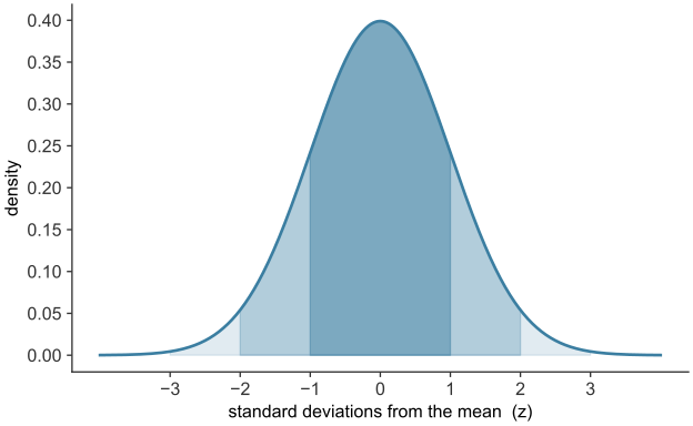
Figure 27.7: The standard normal density, shaded within 1, 2, and 3 standard deviations of the mean. Generated by scripts/03_statistics/06_binomial_and_normal/gen_binomial_and_normal.py.

The areas are \(68.3\%\) within one standard deviation of the mean, \(95.4\%\) within two, and \(99.7\%\) within three (see Figure 27.7). Rounded, they give the 68–95–99.7 rule: about \(68\%\) of a normal distribution’s values fall within one standard deviation of the mean, about \(95\%\) within two, and about \(99.7\%\) within three. ::::: {.callout-important .knowledge-check icon=“false”} ## Knowledge check

A population of recovery times is modeled as normal with mean \(\mu = 50\) days and standard deviation \(\sigma = 8\) days. (a) What is the z-score of a recovery time of \(66\) days? (b) Using the \(68\)–\(95\)–\(99.7\) rule, about what fraction of patients recover within \(66\) days?

NoteAnswer

1. \(z = (66-50)/8 = 16/8 = 2\): the value is exactly two standard deviations above the mean.

2. About \(95\%\) of the distribution lies within two standard deviations of the mean, split evenly by symmetry into about \(47.5\%\) below \(\mu\) and \(47.5\%\) above. Adding the \(50\%\) below the mean itself, about \(50\% + 47.5\% = 97.5\%\) of patients recover within \(66\) days. Equivalently, about \(2.5\%\) take longer.

:::::

Normal approximation to the binomial

A binomial probability with a large \(n\) is a long sum. The probability of \(45\) or fewer heads in \(100\) fair flips adds \(46\) terms. The normal curve gives an answer from one table lookup when the rule of thumb below is met. For a binomial count, the normal model uses the binomial’s own mean and standard deviation:

\[ \mu = np, \qquad \sigma = \sqrt{np(1-p)}. \]

At \(n = 10\) the bars pile up against zero, and the normal curve fits them poorly. As \(n\) grows, the bars fill out a symmetric bell, and the normal curve fits them closely (see Figure 27.8).

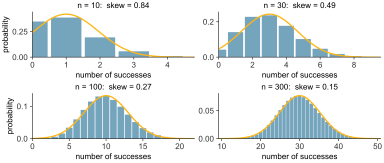
Figure 27.8: Binomial distributions with \(p = 0.1\) for \(n = 10, 30, 100, 300\) (bars), with the normal curve of the same mean and standard deviation (gold). The title gives the skewness, \((1-2p)/\sqrt{np(1-p)}\). Generated by scripts/03_statistics/06_binomial_and_normal/gen_binomial_and_normal.py.

NoteNormal approximation of the binomial distribution

As a general rule, the binomial is well approximated by a normal curve when \(np \geq 10\) and \(n(1-p) \geq 10\). The normal curve takes the binomial’s mean and standard deviation.

Take \(100\) flips of a fair coin. Here \(np = 50\) and \(n(1-p) = 50\), so the rule is met, and the normal model is \(N(50,\ 5)\) (see Figure 27.9).

n, p = 100, 0.5
mean = n * p
sd = (n * p * (1 - p)) ** 0.5
print(f"np = {mean:.1f}, n(1-p) = {n*(1-p):.1f}  (both >= 10)")

np = 50.0, n(1-p) = 50.0  (both >= 10)

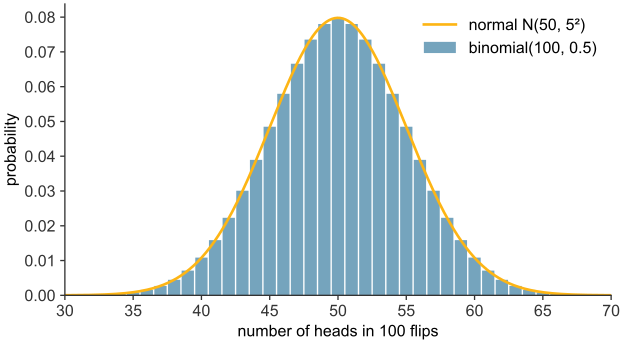
Figure 27.9: Probability of each number of heads in \(100\) fair flips (bars), with the normal approximation \(N(50,\ 5)\) (curve). Generated by scripts/03_statistics/06_binomial_and_normal/gen_binomial_and_normal.py.

Find \(P(X \le 45)\). The exact binomial sum is \(0.184\). The count takes whole values, so the normal cutoff is moved halfway to the next value, to \(45.5\). The normal curve then gives \(z = (45.5 - 50)/5 = -0.9\) and a probability of \(0.184\).

Application: the Dermagraft trial

Take the healing rate of the device arm as known, \(p = 0.300\), with \(130\) patients. Then \(np = 39.0\) and \(n(1-p) = 91.0\), so the rule is met, and the normal model is \(N(39.0,\ 5.22)\).

The probability that \(39\) or fewer patients heal is \(0.543\) exactly. The normal curve, with the cutoff moved to \(39.5\), gives \(z = (39.5 - 39.0)/5.22 \approx 0.096\) and a probability of \(0.538\), within \(0.005\) of the exact value.

TipProblem 1

A new wound-care device is tested on \(n = 50\) independent patients, each with assumed true healing probability \(p = 0.4\).

1. Identify the four conditions that must hold for the binomial model to apply here, and confirm each is plausible.
2. Compute the mean and standard deviation of the number who heal.
3. Compute \(P(X = 20)\) using the binomial formula.

NoteAnswer 1

1. The trials must be independent (patients do not affect each other’s healing), the number fixed in advance (\(n=50\)), each outcome a clear success or failure (heal / not heal), and the success probability the same for every patient (\(p=0.4\)). All four are plausible for one treatment arm of unrelated patients enrolled under the same protocol.

2. \(\mu = np = 50 \times 0.4 = 20\); \(\sigma = \sqrt{np(1-p)} = \sqrt{50 \times 0.4 \times 0.6} = \sqrt{12} \approx 3.46\).

3. \(P(X=20) = \binom{50}{20}(0.4)^{20}(0.6)^{30} \approx 0.115\).

TipProblem 2

Show algebraically that the variance of a binomial random variable, \(\sigma_X^2 = np(1-p)\), follows from treating \(X\) as a sum of \(n\) independent \(0\)/\(1\) variables, each with variance \(p(1-p)\).

NoteAnswer 2

Write \(X = Y_1 + Y_2 + \cdots + Y_n\), where each \(Y_i\) is the \(0\)/\(1\) outcome of trial \(i\), with \(\mathrm{Var}(Y_i) = p(1-p)\). Because the trials are independent, the variance of their sum is the sum of their variances:

\[ \mathrm{Var}(X) = \mathrm{Var}(Y_1) + \cdots + \mathrm{Var}(Y_n) = \underbrace{p(1-p) + \cdots + p(1-p)}_{n \text{ terms}} = n\,p(1-p). \]

TipProblem 3

A patient’s post-operative recovery time is modeled as normal with mean \(\mu = 40\) days and standard deviation \(\sigma = 6\) days.

1. Compute the z-score for a recovery time of \(28\) days.
2. Compute the z-score for a recovery time of \(49\) days.
3. Which of the two recovery times is more unusual, and why?

NoteAnswer 3

1. \(z = (28-40)/6 = -12/6 = -2\).

2. \(z = (49-40)/6 = 9/6 = 1.5\).

3. The \(28\)-day recovery is more unusual. Its z-score has the larger absolute value, \(|-2| > |1.5|\), so it lies further from the mean in standard deviations, although \(49\) days is further from the mean in raw days.

TipProblem 4

For the Dermagraft control arm, \(n = 115\) and \(p = 0.183\).

1. Compute \(np\) and \(n(1-p)\), and check whether the normal approximation to the binomial is appropriate.
2. Give the mean and standard deviation of the approximating normal distribution.
3. Using the \(68\)–\(95\)–\(99.7\) rule and your answer to (b), give an interval that should contain the number of healed ulcers in about \(95\%\) of repeated trials of this size.

NoteAnswer 4

1. \(np = 115 \times 0.183 \approx 21.0\) and \(n(1-p) = 115 \times 0.817 \approx 94.0\). Both exceed \(10\), so the normal approximation is appropriate.

2. \(\mu = 21.0\); \(\sigma = \sqrt{115 \times 0.183 \times 0.817} \approx \sqrt{17.2} \approx 4.15\).

3. About \(95\%\) of the distribution falls within \(2\sigma \approx 8.3\) of the mean, giving the interval \(21.0 \pm 8.3 \approx [12.7,\ 29.3]\) healed ulcers.

TipProblem 5

A rare complication occurs independently in each patient with probability \(p = 0.02\). A study enrolls \(n = 40\) patients.

1. Compute \(np\) and \(n(1-p)\).
2. Is the normal approximation to the binomial appropriate here? Explain using the rule of thumb.
3. What does this suggest about using a normal model for rare events observed in small-to-moderate samples?

NoteAnswer 5

1. \(np = 40 \times 0.02 = 0.8\); \(n(1-p) = 40 \times 0.98 = 39.2\).

2. No. Although \(n(1-p)\) is large, \(np = 0.8\) is far below the required \(10\), so the rule of thumb fails and the normal approximation should not be used here.

3. When an event is rare, \(np\) stays small even for a moderately large \(n\), so a much larger sample is needed before the count of occurrences is well approximated by a normal curve. For rare complications the binomial formula should be used directly rather than the normal approximation.

NoteFurther reading

• Diez, Çetinkaya-Rundel and Barr, OpenIntro Statistics, 4th ed. A free open textbook covering the topics of this chapter (Diez et al. 2019).

References

Diez, David M., Mine Çetinkaya-Rundel, and Christopher D. Barr. 2019. OpenIntro Statistics. 4th ed. OpenIntro. https://www.openintro.org/book/os/.