28 Sampling and the Sampling Distribution
A trial measures a sample and computes a statistic from it: a sample mean \(\bar{x}\), a healing rate. But the quantity of interest is a parameter of the whole population: the fixed but unknown \(\mu\) the sample was meant to estimate. The statistic is also variable: a different sample would have produced a different \(\bar{x}\). The gap between a statistic and its parameter is measured by how far the statistic tends to stray, and how that gap closes as the sample grows.
A statistic computed from a random sample has a distribution of its own, the sampling distribution, traced out over all the samples that might have been drawn. Three facts about that distribution allow a single sample to estimate a population it does not fully measure. It centers on the parameter (the Law of Large Numbers). Its spread shrinks as \(\sigma/\sqrt{n}\) (the standard error). Its shape approaches a normal curve regardless of the population’s shape (the Central Limit Theorem). Together these facts justify applying the 68–95–99.7 rule to a sample mean, and the standard-error formula \(\mathrm{SE} = \sqrt{p(1-p)/n}\) for a rate such as the Dermagraft healing rates.
A population that can be measured in full
In a real study, the population is out of reach. A trial enrolls a hundred patients but its conclusion is meant to hold for all patients who might ever be treated. The true rate among them can never be seen. Where the whole population is available, a sample statistic can be checked against the parameter it estimates.
The example is a record of United Airlines domestic flights leaving San Francisco in the summer of \(2015\): \(13{,}825\) flights, each with its departure delay in minutes, compiled from U.S. Bureau of Transportation Statistics records and distributed with the Data 8 course materials (Adhikari et al. 2022). A negative delay marks a flight that left early. These \(13{,}825\) flights are the population. Their mean, median, and standard deviation are population parameters, known exactly.
united = pd.read_csv(DATA + "united_summer2015.csv")
delay = united["Delay"].to_numpy()          # departure delay, in minutes

N = delay.size
mu = delay.mean()                            # population mean  mu   (a parameter)
sigma = delay.std(ddof=0)                    # population SD    sigma (a parameter)

print(f"population size   N     = {N:,} flights")
print(f"mean delay        mu    = {mu:.2f} min")
print(f"median delay             = {np.median(delay):.0f} min")
print(f"std of delays     sigma = {sigma:.2f} min")
print(f"range                    = {delay.min()} to {delay.max()} min")
print(f"delays over 200 min      = {(delay > 200).mean()*100:.1f}% of flights")
population size N = 13,825 flights
mean delay mu = 16.66 min
median delay = 2 min
std of delays sigma = 39.48 min
range = -16 to 580 min
delays over 200 min = 0.8% of flightsThe population is strongly right-skewed (see Figure 28.1). Most flights leave close to on time; the median delay is \(2\) minutes. But a thin tail of badly delayed flights, a few of them by hours, drags the mean up to \(\mu = 16.7\) minutes, above the median. Fewer than one flight in a hundred is delayed beyond \(200\) minutes.
bins = np.arange(-20, 201, 10)          # 10-minute bins across the bulk of the data

fig, ax = plt.subplots()
ax.hist(delay, bins=bins, density=True, color=BLUE, edgecolor="white")
ax.axvline(mu, color=GOLD, lw=2, label=f"population mean  μ = {mu:.1f} min")
ax.set_xlabel("departure delay (minutes)")
ax.set_ylabel("proportion per minute (density)")
ax.legend()
plt.show()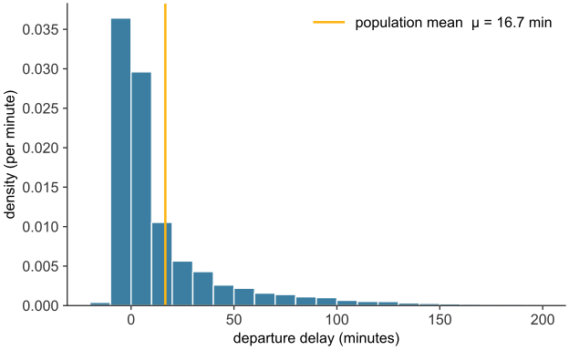
scripts/03_statistics/07_sampling_distribution/gen_sampling_distribution.py.
The histogram uses the density scale from numerical data: the area of each bar is the proportion of flights it holds, and the total area is \(1\). This lets histograms of different numbers of flights be compared directly.
Drawing a random sample
A sample is a subset of the population actually observed. A random sample is one in which chance alone chooses the members, each flight having a known, equal chance of selection. A sample assembled by any rule tied to the delay itself (the first flights of the day, the flights an analyst happened to notice) could systematically over- or understate the delays. A random sample has no such leaning, so its departures from the population are chance errors. In pandas, DataFrame.sample draws one; fixing random_state makes the particular draw reproducible.
# A random sample of 10 of the 13,825 flights (random_state fixes the draw).
united.sample(10, random_state=0)[["Date", "Flight Number", "Destination", "Delay"]]
Date Flight Number Destination Delay
7/21/15 1796 IAD 3
6/18/15 1723 KOA 12
8/15/15 1946 BOS 15
6/13/15 1726 LAS 8
6/19/15 1526 DEN 8
7/28/15 401 CLE 1
6/20/15 73 HNL 331
6/5/15 1614 LAS 1
6/17/15 760 JFK -4
6/30/15 758 JFK 9Sampling without replacement removes each flight as it is picked, so no flight appears twice. This is the model of a survey, in which a person is not polled twice. Sampling with replacement returns each flight before the next is drawn, so the draws are independent and identical, each from the full population. When the sample is small beside the population (ten flights out of \(13{,}825\)), the two are practically indistinguishable.
What a large sample looks like
A random sample resembles its population more closely as it grows. Histograms of random samples of \(100\) flights and of \(2{,}000\), each against the outline of the population, illustrate this (see Figure 28.2).
fig, axes = plt.subplots(1, 2, figsize=(9.5, 3.8), sharey=True)
for ax, n in zip(axes, [100, 2000]):
    sample = united["Delay"].sample(n, replace=True, random_state=1).to_numpy()
    ax.hist(sample, bins=bins, density=True, color=BLUE, edgecolor="white",
            label=f"sample of {n:,}")
    ax.hist(delay, bins=bins, density=True, histtype="step",
            color=GOLD, lw=2, label="population")
    ax.set_xlabel("delay (minutes)")
    ax.legend()
axes[0].set_ylabel("density")
fig.tight_layout()
plt.show()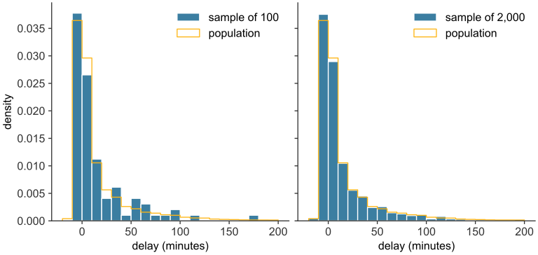
scripts/03_statistics/07_sampling_distribution/gen_sampling_distribution.py.
The sample of \(100\) has the same skewed shape, but its bars run above and below the population outline. The sample of \(2{,}000\) follows the outline closely.
The sampling distribution of the mean
A statistic computed from a large sample, the sample mean \(\bar{x}\), should fall near the corresponding parameter \(\mu\). Drawing five separate samples of the same size gives five different sample means.
rng = np.random.default_rng(1)
sample_means = [rng.choice(delay, size=400, replace=True).mean() for _ in range(5)]
print("means of five separate random samples, each of n = 400 flights:")
print("  " + ",  ".join(f"{m:.1f}" for m in sample_means) + "  minutes")
means of five separate random samples, each of n = 400 flights:
15.0, 17.0, 17.7, 15.4, 17.0 minutesThe five sample means cluster near the population mean of \(16.7\) minutes, and none equals it exactly. The sample mean is therefore a random quantity, and like any random quantity it has a distribution. The sampling distribution of a statistic is the distribution of its values over all the samples that might have been drawn.
Enumerating all possible samples is not feasible, so the sampling distribution is approximated instead. Drawing many thousands of samples, computing the mean of each, and building a histogram of those means yields an empirical sampling distribution that resembles the true one, more closely as more samples are drawn.
def sampling_distribution(n, reps=10_000, seed=7):
    """Return the means of `reps` random samples, each of size n (with replacement)."""
    rng = np.random.default_rng(seed)
    return np.array([rng.choice(delay, size=n, replace=True).mean()
                     for _ in range(reps)])

def normal_pdf(x, m, s):
    """Normal probability density with mean m and standard deviation s."""
    return np.exp(-0.5 * ((x - m) / s) ** 2) / (s * np.sqrt(2 * np.pi))

fig, axes = plt.subplots(1, 3, figsize=(11, 3.6))
for ax, n in zip(axes, [4, 100, 400]):
    means = sampling_distribution(n)
    se = sigma / np.sqrt(n)                       # predicted standard error
    ax.hist(means, bins=40, density=True, color=BLUE, edgecolor="white")
    grid = np.linspace(means.min(), means.max(), 200)
    ax.plot(grid, normal_pdf(grid, mu, se), color=GOLD, lw=2,
            label="normal N(μ, σ²/n)")
    ax.axvline(mu, color=GREEN, lw=1.5, ls="--", label="population mean μ")
    ax.set_title(f"n = {n}     SE = σ/√n = {se:.1f} min")
    ax.set_xlabel("sample mean delay (min)")
    print(f"n = {n:>3}:  mean of sample means = {means.mean():5.2f} min   "
          f"SD of sample means = {means.std(ddof=0):5.2f} min   "
          f"sigma/sqrt(n) = {se:5.2f} min")
axes[0].set_ylabel("density")
axes[2].legend(fontsize=8)
fig.tight_layout()
plt.show()
n = 4: mean of sample means = 16.64 min SD of sample means = 19.63 min sigma/sqrt(n) = 19.74 min
n = 100: mean of sample means = 16.66 min SD of sample means = 3.98 min sigma/sqrt(n) = 3.95 min
n = 400: mean of sample means = 16.65 min SD of sample means = 1.97 min sigma/sqrt(n) = 1.97 min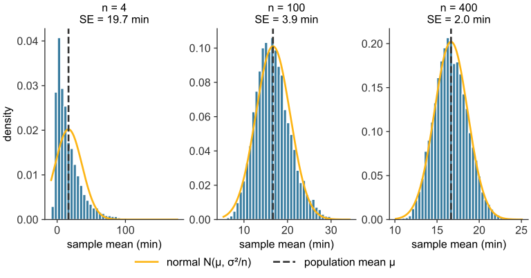
scripts/03_statistics/07_sampling_distribution/gen_sampling_distribution.py.
Each of the three histograms summarizes the sample means of ten thousand samples (see Figure 28.3). The orange curve is the normal curve \(N(\mu,\ \sigma^2/n)\), and the dashed line marks the population mean.
Skewness measures asymmetry. It is \(0\) for a symmetric distribution and positive when the long tail lies on the right. The skewness of the simulated sample means is about \(2.0\) at \(n = 4\), \(0.5\) at \(n = 100\), and \(0.2\) at \(n = 400\).
The Law of Large Numbers and the Central Limit Theorem
The Law of Large Numbers states that the sample mean \(\bar{X}\) converges to the population mean \(\mu\) as the sample size \(n\) grows without bound. The Central Limit Theorem describes the shape of \(\bar{X}\) before that limit is reached. For independent observations from a population with mean \(\mu\) and standard deviation \(\sigma\), the distribution of \(\bar{X}\) is approximately normal when \(n\) is sufficiently large, with standard deviation \(\sigma/\sqrt{n}\). The population need not be normal. A common rule of thumb is \(n \ge 30\), provided the sample has no extreme outliers (Diez et al. 2019).
\[ \bar{X} \;\approx\; N\!\left(\mu,\ \frac{\sigma^2}{n}\right) \qquad \text{for large } n. \]
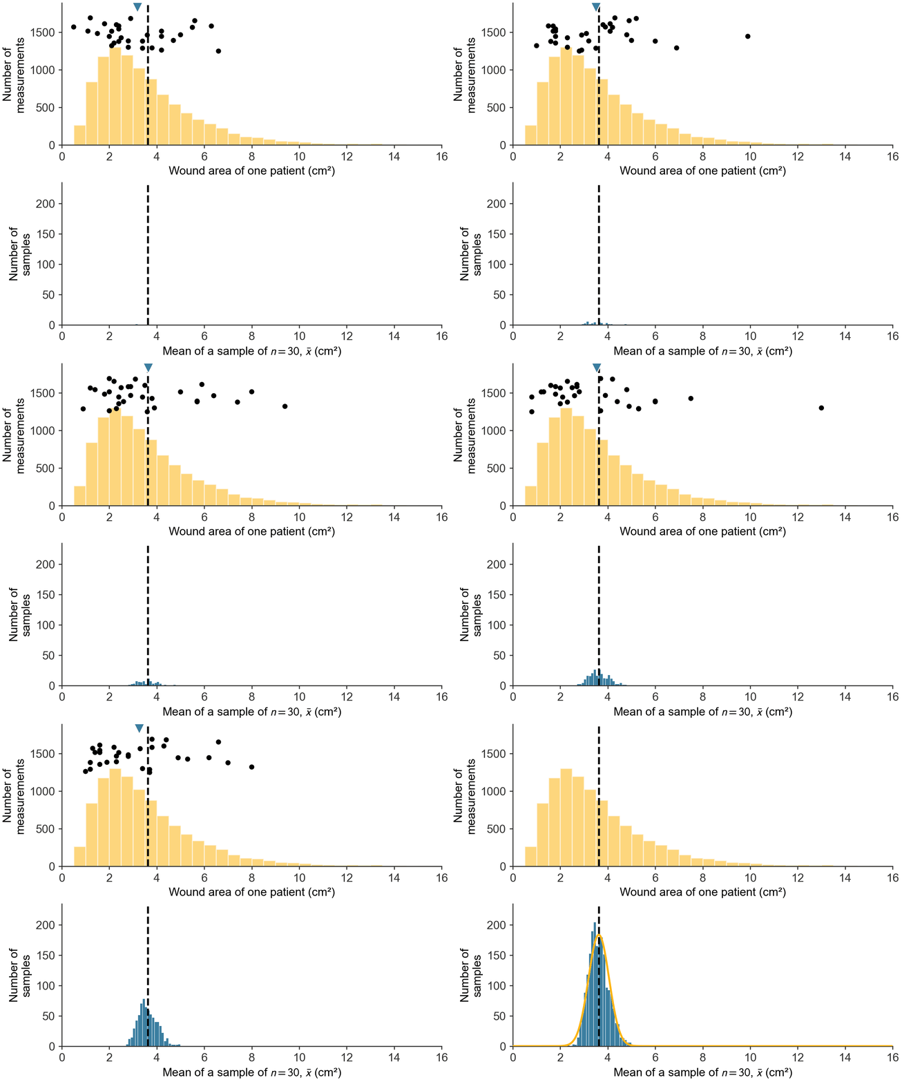
Each sample of \(30\) values is marked on the population, and its mean drops into a histogram of sample means (see Figure 28.4). After \(2{,}000\) samples, the normal curve appears over the histogram, and the bell shape emerges as \(n\) grows across four sample sizes (see Figure 28.5).
scripts/03_statistics/07_sampling_distribution/gen_clt_animations.py.
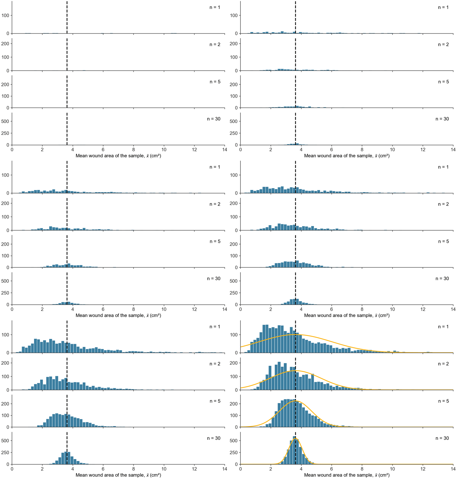
scripts/03_statistics/07_sampling_distribution/gen_clt_animations.py.
The population in Figure 28.6 is strongly right-skewed: most values are small, and a few are large. Its mean is \(\mu = 3\) and its standard deviation is \(\sigma = 3\). Move the slider to change the sample size \(n\). For each \(n\), the figure draws \(2{,}000\) samples and plots their means. As \(n\) grows, the histogram of means becomes a bell curve, centered on \(\mu\), with width \(\sigma/\sqrt{n}\).
The standard error and the \(1/\sqrt{n}\) law
The standard deviation of a sampling distribution is called the standard error, to distinguish it from the population standard deviation \(\sigma\). It is the typical distance between a sample mean and the population mean. The simulation agrees: at \(n = 100\) the ten thousand sample means scattered with standard deviation \(3.98\) minutes against a predicted \(\sigma/\sqrt{n} = 3.95\); at \(n = 400\), \(1.97\) against \(1.97\).
Because the standard error falls as the square root of \(n\), precision improves at a diminishing rate: to halve the standard error one must quadruple the sample. Going from \(n = 100\) to \(n = 400\) (four times the data) cuts the standard error from \(3.95\) to \(1.97\) minutes, a factor of two. Halving it once more would take \(1{,}600\) flights.
For a proportion, \(\mathrm{SE} = \sqrt{p(1-p)/n}\) gives the standard error of the Dermagraft rates.
def bernoulli_se(p, n):
    """Standard error of a proportion (rate) p observed in a sample of size n."""
    return np.sqrt(p * (1 - p) / n)

print(f"device  arm:  p = 0.300, n = 130  ->  SE = {bernoulli_se(0.300, 130)*100:.1f} percentage points")
print(f"control arm:  p = 0.183, n = 115  ->  SE = {bernoulli_se(0.183, 115)*100:.1f} percentage points")
print(f"15-patient pilot at p = 0.300      ->  SE = {bernoulli_se(0.300, 15)*100:.1f} percentage points")
device arm: p = 0.300, n = 130 -> SE = 4.0 percentage points
control arm: p = 0.183, n = 115 -> SE = 3.6 percentage points
15-patient pilot at p = 0.300 -> SE = 11.8 percentage pointsAt the trial’s enrollment (\(130\) patients on the device, \(115\) on standard care), each healing rate has a standard error of about \(4\) percentage points, so the \(11.7\)-point difference between \(30.0\%\) and \(18.3\%\) is larger than the standard error of either rate. In a \(15\)-patient pilot, the standard error of each rate is \(11.8\) points, about equal to the difference, so chance alone could produce a difference that size. The hypothesis test decides formally how many standard errors of separation count as convincing.
Turning the standard error into a probability
The Central Limit Theorem gives the sampling distribution a normal shape, so the 68–95–99.7 rule applies to it. For large \(n\), a sample mean is normally distributed about \(\mu\) with standard deviation \(\mathrm{SE}\), so about \(95\%\) of samples of size \(n\) produce a mean within \(2\,\mathrm{SE}\) of \(\mu\). For the flight delays at \(n = 400\), where \(\mathrm{SE} = 2.0\) minutes, roughly \(95\%\) of sample means land within \(4\) minutes of \(\mu = 16.7\).
A sample mean \(\bar{x}\) observed against a hypothesized population mean \(\mu\) has z-score \(z = (\bar{x} - \mu)/\mathrm{SE}\), counting the standard errors between them. A \(z\) near \(0\) means the sample mean lies close to the hypothesized \(\mu\). A \(z\) beyond \(\pm 2\) occurs in about \(5\%\) of samples when the hypothesized \(\mu\) is the true mean.
Exercises
References
Adhikari, Ani, John DeNero, and David Wagner. 2022. Computational and Inferential Thinking: The Foundations of Data Science. 2nd ed. University of California, Berkeley (Data 8). https://inferentialthinking.com/.
Diez, David M., Mine Çetinkaya-Rundel, and Christopher D. Barr. 2019. OpenIntro Statistics. 4th ed. OpenIntro. https://www.openintro.org/book/os/.