7  Simplified Bernoulli

To apply the Bernoulli equation, consider blood flowing through a heart valve.
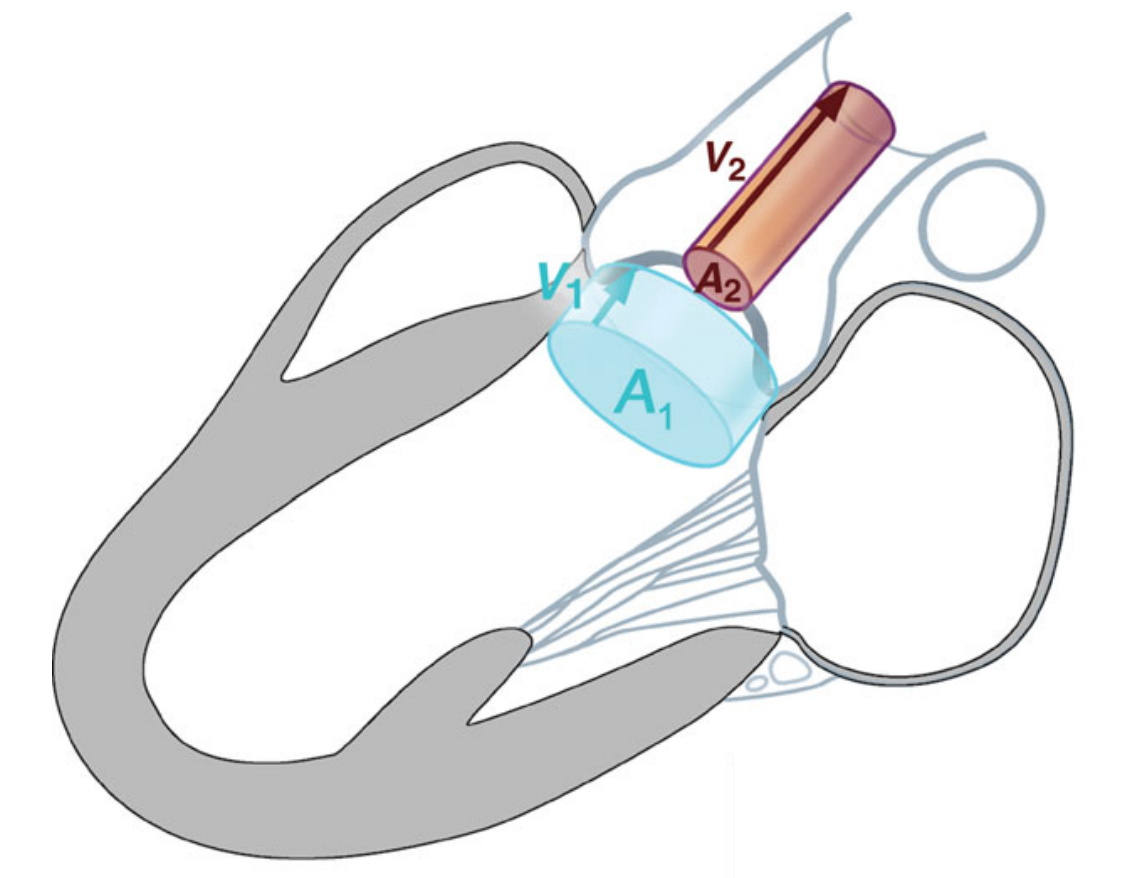
Figure 7.1: A simplified view of the blood flow through a heart valve.

Point 1 lies in the chamber just upstream of the valve, where the blood moves slowly at \(v_1\), and point 2 lies in the narrow jet through the valve, where continuity has raised the speed to \(v_2\). Under the assumptions of steady, frictionless flow along a streamline established previously, Bernoulli’s equation relates the pressure and velocity at these points:

\[P_1 + \tfrac{1}{2}\rho v_1^2 + \rho g h_1 = P_2 + \tfrac{1}{2}\rho v_2^2 + \rho g h_2 .\]

The quantity of interest is the pressure drop \(\Delta p = P_1 - P_2\) that the heart must supply.

Step 1 — the valve is horizontal. The two sides of a valve lie at essentially the same height, so \(h_1 \approx h_2\) and the two \(\rho g h\) terms cancel — a simplification, since the two sides are not in fact at exactly the same height. Rearranging the remainder,

\[\Delta p = P_1 - P_2 = \tfrac{1}{2}\rho\big(v_2^2 - v_1^2\big).\]

Step 2 — the upstream speed is negligible. By continuity the wide chamber feeds a narrow orifice, so \(v_2 \gg v_1\); and because the velocities enter the equation squared, the velocity at point 2 dominates the difference. Dropping the small \(v_1^2\) and writing the jet speed as \(v_{\max}\) (the peak velocity reported by the ultrasound),

\[\Delta p \approx \tfrac{1}{2}\rho\,v_{\max}^2 .\]

Step 3 — insert the density and convert the units. Blood has density \(\rho \approx 1060~\text{kg/m}^3\), a standard physiological value slightly above water’s \(1000\). With \(v_{\max}\) in meters per second, this gives \(\Delta p\) in pascals:

\[\Delta p \approx \tfrac{1}{2}(1060)\,v_{\max}^2 = 530\,v_{\max}^2~\text{Pa}.\]

Clinicians, however, quote pressure in mmHg rather than pascals, and the conversion is \(1~\text{mmHg} = 133.3~\text{Pa}\). Dividing,

\[\Delta p~[\text{mmHg}] \approx \frac{530\,v_{\max}^2}{133.3} = 3.98\,v_{\max}^2 \approx 4\,v_{\max}^2 .\]

The origin of the “4” is now explicit: it is \(\tfrac{1}{2}\rho / 133.3 = \tfrac{1}{2}(1060)/133.3 = 3.98\), rounded for clinical use. The constant incorporates the density of blood and the pascal-to-mmHg conversion, so it is specific to cardiology; the same calculation with the density of water gives 3.75 rather than 4.

NoteKey result: the simplified Bernoulli equation

For blood passing through a narrowed heart valve, the pressure gradient the heart must generate is determined by the jet’s peak velocity alone:

\[\boxed{\;\Delta p \approx 4\,v_{\max}^2\;} \qquad \left(\Delta p~\text{in mmHg},\quad v_{\max}~\text{in m/s}\right).\]

Measuring the jet velocity with Doppler ultrasound, squaring it, and multiplying by four gives the pressure drop across the valve in the units a cardiologist uses, without any instrument entering the body (Heys et al. 2010). The formula rests on the three assumptions made explicitly above: the flow is frictionless, the valve is horizontal, and the upstream velocity is negligible.

WarningWhere the approximation breaks down
  • Viscous losses are ignored. A real stenotic jet dissipates some energy to friction, energy that the frictionless Bernoulli equation assumes is available to convert into pressure. The simplified formula therefore tends to overestimate the true gradient in some settings.
  • The upstream velocity is neglected. Dropping \(v_1\) is excellent when \(v_2 \gg v_1\), but if the chamber velocity is not small — a high-output state, or a second narrowing upstream — the full form \(\Delta p = \tfrac{1}{2}\rho(v_2^2 - v_1^2)\) should be used instead.
  • Steady flow is assumed. Cardiac flow is pulsatile, not steady, and an additional acceleration term may be needed in some cases.
  • \(v_{\max}\) must be the true peak. Doppler reports only the velocity component along the beam, \(v\cos\theta\); a misaligned beam under-reads the velocity, and because \(\Delta p \propto v^2\), that error is squared into a substantially larger under-estimate of the gradient.

The simplified formula is therefore a useful clinical estimate rather than an exact energy balance, and its accuracy depends on how closely the three assumptions above hold for a given patient.

ImportantKnowledge check

A diseased valve has narrowed to one-third of its healthy opening area, while the heart still drives the same volumetric flow \(Q\) through it. By what factor does the jet velocity rise, and by what factor does the pressure gradient \(\Delta p\) across the valve grow?

By continuity \(A v = Q\) is fixed, so shrinking the area to one-third forces the velocity up by a factor of 3 (\(v = Q/A\), and \(A\) fell to a third). The gradient follows \(\Delta p \approx 4v^2\), which depends on velocity squared, so tripling \(v\) multiplies \(\Delta p\) by \(3^2 = \mathbf{9}\). A modest reduction in area therefore produces a disproportionately large pressure load; this steep, quadratic dependence is why stenosis places such a burden on the heart.

A stenotic mitral valve

The mitral valve is the left-heart atrioventricular valve, through which blood passes to fill the left ventricle. Take a healthy mitral valve whose peak inflow velocity is a normal \(v_{\text{healthy}} = 1~\text{m/s}\), and compare it with a stenotic valve whose opening has narrowed to half its healthy area while the heart drives the same flow \(Q\) through it. The code below performs both calculations and plots the result.

import numpy as np
import matplotlib.pyplot as plt
plt.style.use("../../theme/bioe10.mplstyle")

RHO  = 1060.0            # blood density, kg/m^3
MMHG = 133.322           # pascals per mmHg

def dp_mmHg(v):          # simplified Bernoulli: v in m/s -> pressure gradient in mmHg
    return 0.5 * RHO * v**2 / MMHG

# healthy valve: normal peak inflow velocity
v_healthy = 1.0
# stenotic valve: HALF the area at the same flow Q -> continuity DOUBLES the velocity
v_stenotic = v_healthy * (1 / 0.5)      # A -> A/2, so v -> 2v

print(f"coefficient 0.5*rho/mmHg = {0.5 * RHO / MMHG:.3f}  (the clinical '4')")
print(f"healthy : v = {v_healthy:.1f} m/s -> dp = {dp_mmHg(v_healthy):.1f} mmHg")
print(f"stenotic: v = {v_stenotic:.1f} m/s -> dp = {dp_mmHg(v_stenotic):.1f} mmHg")
print(f"gradient grew by {dp_mmHg(v_stenotic) / dp_mmHg(v_healthy):.0f}x")

fig, (axA, axB) = plt.subplots(1, 2, figsize=(10, 4.2))

# Panel A -- continuity: velocity vs orifice area (constant flow), v = v_healthy / frac
frac = np.linspace(0.30, 1.05, 200)          # orifice area as a fraction of healthy
axA.plot(frac, v_healthy / frac, color="#0072B2")
axA.scatter([1.0, 0.5], [v_healthy, v_stenotic], color=["#333333", "#D55E00"], zorder=5)
axA.annotate("healthy", (1.0, v_healthy), textcoords="offset points", xytext=(8, -14))
axA.annotate("stenotic", (0.5, v_stenotic), textcoords="offset points",
             xytext=(-40, 16), ha="right", color="#D55E00")
axA.set_xlabel("orifice area (fraction of healthy)")
axA.set_ylabel("jet velocity (m/s)")

# Panel B -- Bernoulli: pressure gradient vs velocity, dp = 4 v^2
v = np.linspace(0, 3, 200)
axB.plot(v, dp_mmHg(v), color="#E69F00")
axB.scatter([v_healthy, v_stenotic],
            [dp_mmHg(v_healthy), dp_mmHg(v_stenotic)], color=["#333333", "#D55E00"], zorder=5)
axB.annotate("healthy", (v_healthy, dp_mmHg(v_healthy)), textcoords="offset points",
             xytext=(-10, 10), ha="right")
axB.annotate("stenotic", (v_stenotic, dp_mmHg(v_stenotic)), textcoords="offset points",
             xytext=(-10, -18), ha="right", color="#D55E00")
axB.text(0.15, dp_mmHg(v).max() * 0.9, r"$\Delta p \approx 4v^2$", fontsize=12)
axB.set_xlabel("jet velocity (m/s)")
axB.set_ylabel(r"pressure gradient $\Delta p$ (mmHg)")

plt.show()

Running the code prints

coefficient 0.5*rho/mmHg = 3.975  (the clinical '4')
healthy : v = 1.0 m/s -> dp = 4.0 mmHg
stenotic: v = 2.0 m/s -> dp = 15.9 mmHg
gradient grew by 4x

and produces Figure 7.2.
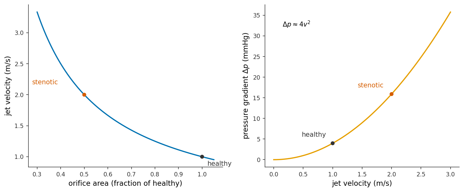
Figure 7.2: The stenosis chain for a mitral valve. Left (continuity): at a fixed flow, jet velocity climbs as the orifice area shrinks; halving the area (black → red) doubles the velocity from 1 to 2 m/s. Right (Bernoulli): the pressure gradient follows \(\Delta p \approx 4v^2\), so that doubled velocity quadruples the gradient, from about 4 to about 16 mmHg. Generated by the code above.

Doppler to pressure

The ultrasound reports a blood velocity from the Doppler shift of a returning echo, \(v = c f_D / (2 f_0 \cos\theta)\). The clinically required quantity, however, is not velocity but the pressure gradient a stenotic valve imposes on the heart. Conservation of mass and conservation of energy supplied the two physical laws needed to derive Bernoulli’s equation, and the simplification above produced a clinical rule. The full noninvasive chain is:

\[\underbrace{f_D}_{\text{measured}} \;\xrightarrow{\;v = c f_D / 2 f_0\cos\theta\;}\; \underbrace{v_{\max}}_{\text{blood-jet speed}} \;\xrightarrow{\;\Delta p \approx 4 v_{\max}^2\;}\; \underbrace{\Delta p}_{\text{valve pressure gradient}} .\]

A cardiac probe transmits at \(f_0 = 2.0~\text{MHz}\), aligned nearly along an aortic-valve jet (\(\theta \approx 0\)), and the returning echo is shifted by \(f_D = 10.4~\text{kHz}\). The code below converts Doppler shift to velocity and then applies the simplified Bernoulli equation.

import numpy as np

c    = 1540.0           # speed of sound in tissue, m/s
RHO  = 1060.0           # blood density, kg/m^3
MMHG = 133.322          # pascals per mmHg

f0  = 2.0e6             # transmitted frequency, Hz
fD  = 10.4e3            # measured Doppler shift, Hz
ct  = 1.0               # cos(theta), beam aligned with the jet

# Step 1 -- Doppler: frequency shift -> blood-jet velocity
v = c * fD / (2 * f0 * ct)
print(f"blood-jet velocity  v   = {v:.2f} m/s")

# Step 2 -- Bernoulli: velocity -> valve pressure gradient
dp = 4 * v**2                       # clinical rule, mmHg
dp_exact = 0.5 * RHO * v**2 / MMHG  # the un-rounded version, for comparison
print(f"pressure gradient   dp  = {dp:.0f} mmHg  (exact {dp_exact:.1f} mmHg)")

which prints

blood-jet velocity  v   = 4.00 m/s
pressure gradient   dp  = 64 mmHg  (exact 63.7 mmHg)

The 10.4 kHz shift implies a jet velocity of 4 m/s, and a pressure gradient of about 64 mmHg across the valve: the left ventricle must generate an additional 64 mmHg on every beat to drive blood through the narrowed opening.

Exercises

TipProblem 1

A Doppler ultrasound reports the peak velocity of the jet crossing a patient’s aortic valve.

  1. For a patient whose jet peaks at \(v_{\max} = 3.5~\text{m/s}\), estimate the pressure gradient \(\Delta p\) across the valve using the simplified Bernoulli equation.
  2. A second patient’s gradient is measured a different way and comes out at \(\Delta p = 64~\text{mmHg}\). What peak jet velocity does that imply?
  1. \(\Delta p \approx 4 v_{\max}^2 = 4 (3.5)^2 = 4 (12.25) = \mathbf{49~mmHg}\).

  2. Invert the formula: \(v_{\max} = \sqrt{\Delta p / 4} = \sqrt{64/4} = \sqrt{16} = \mathbf{4~m/s}\). (Both gradients are large — the sort of number that flags a significantly narrowed aortic valve.)

TipProblem 2

In the worked example we halved the valve’s area. Real narrowings are often described by diameter instead. Suppose a stenotic valve has half the diameter of a healthy one, and the heart drives the same flow \(Q\) through it. Treating the orifice as a circle,

  1. by what factor does the opening area change?
  2. by what factor does the jet velocity change?
  3. by what factor does the pressure gradient \(\Delta p\) change? If the healthy jet was \(1~\text{m/s}\) (gradient \(\approx 4\) mmHg), what is the stenotic gradient?
  1. Area of a circle is \(A = \pi d^2/4\), so \(A \propto d^2\). Halving the diameter multiplies the area by \((1/2)^2 = \mathbf{1/4}\) — a quarter, not a half.

  2. Continuity at fixed \(Q\): \(v \propto 1/A\), so quartering the area multiplies the velocity by \(\mathbf{4}\) (to \(4~\text{m/s}\)).

  3. \(\Delta p \propto v^2\), so the gradient grows by \(4^2 = \mathbf{16}\), from about 4 mmHg to \(4(4)^2 = \mathbf{64~mmHg}\). This is the trap the worked example warned against: halving the diameter is far more severe than halving the area, because area scales as diameter squared and the gradient then scales as area squared.

TipProblem 3

The clinical constant “4” is really a bundle of unit conversions, and this problem takes it apart.

  1. Show that \(\tfrac{1}{2}\rho / (133.3~\text{Pa/mmHg})\) works out to about 4 for blood, \(\rho = 1060~\text{kg/m}^3\).
  2. If you had wrongly used the density of water, \(\rho = 1000~\text{kg/m}^3\), what constant would you get instead?
  3. In one sentence, explain why the clinical rule uses exactly 4 rather than the value you found in (a).
  1. \(\tfrac{1}{2}(1060) = 530\), and \(530 / 133.3 = \mathbf{3.98}\), which rounds to 4.

  2. \(\tfrac{1}{2}(1000) = 500\), and \(500 / 133.3 = \mathbf{3.75}\) — noticeably below 4, which is why the density of blood, not water, has to go into the formula.

  3. The exact coefficient is 3.98; 4 is simply the rounded value, chosen because a whole number is trivial to apply at the bedside and the ~0.5% rounding error is dwarfed by the uncertainty in the measured velocity.

TipProblem 4

The simplified formula throws away the upstream velocity \(v_1\). This problem checks how much that costs. A horizontal valve has upstream speed \(v_1 = 1~\text{m/s}\) and jet speed \(v_2 = 4~\text{m/s}\) (blood, \(\rho = 1060~\text{kg/m}^3\)).

  1. Compute the gradient with the full form \(\Delta p = \tfrac{1}{2}\rho(v_2^2 - v_1^2)\), converted to mmHg.
  2. Compute it with the simplified form \(\Delta p \approx 4 v_2^2\).
  3. By what percentage does dropping \(v_1\) overestimate the gradient here?
  1. \(\Delta p = \tfrac{1}{2}(1060)(4^2 - 1^2) = 530(16 - 1) = 530(15) = 7950~\text{Pa}\). In mmHg, \(7950 / 133.3 = 59.64 \approx \mathbf{59.6~mmHg}\).

  2. \(\Delta p \approx 4(4)^2 = 4(16) = \mathbf{64~mmHg}\).

  3. The overestimate is \((64 - 59.64)/59.64 = 0.073 = \mathbf{7.3\%}\). Neglecting \(v_1\) biases the gradient high, but only modestly when \(v_2 \gg v_1\); the approximation would get worse if the upstream velocity were not so small compared with the jet.

TipProblem 5

Put the whole chain together. A healthy mitral valve has an opening area \(A_0 = 5.0~\text{cm}^2\) and passes blood at a peak velocity \(v_0 = 0.9~\text{m/s}\). Disease narrows the opening to \(A = 1.5~\text{cm}^2\), while the heart drives the same volumetric flow.

  1. Use continuity to find the peak jet velocity through the stenotic valve.
  2. Estimate the pressure gradient across the stenotic valve.
  3. Estimate the gradient across the healthy valve, and state the factor by which stenosis has raised it. Confirm that factor equals \((A_0/A)^2\).
  1. Continuity at fixed flow: \(v = v_0 (A_0/A) = 0.9 \,(5.0/1.5) = 0.9 (3.33) = \mathbf{3.0~m/s}\).

  2. \(\Delta p \approx 4 v^2 = 4 (3.0)^2 = \mathbf{36~mmHg}\).

  3. Healthy: \(\Delta p_0 \approx 4 (0.9)^2 = 4(0.81) = 3.24 \approx \mathbf{3.2~mmHg}\). The ratio is \(36 / 3.24 = \mathbf{11.1}\). Check against the scaling: velocity scales as \(A_0/A\) and \(\Delta p\) as velocity squared, so \(\Delta p\) scales as \((A_0/A)^2 = (5.0/1.5)^2 = (3.33)^2 = 11.1\) — matching exactly.

TipProblem 6

Suppose a clinic flags a mitral valve as concerning once its pressure gradient exceeds \(10~\text{mmHg}\).

  1. What peak jet velocity corresponds to a gradient of exactly 10 mmHg?
  2. The Doppler machine measures velocity to about \(\pm 0.1~\text{m/s}\). Near a jet of \(v = 2~\text{m/s}\), roughly what uncertainty in \(\Delta p\) does that velocity error produce? (Hint: a small input error propagates as \(\Delta y \approx y'\,\Delta x\); here differentiate \(\Delta p = 4v^2\) to get \(d(\Delta p)/dv = 8v\).)
  3. Explain in one sentence why the same \(\pm 0.1~\text{m/s}\) error matters more for a fast jet than a slow one.
  1. \(v_{\max} = \sqrt{\Delta p / 4} = \sqrt{10/4} = \sqrt{2.5} = \mathbf{1.58~m/s}\).

  2. The sensitivity is \(d(\Delta p)/dv = 8v\). At \(v = 2~\text{m/s}\) this is \(8(2) = 16~\text{mmHg per m/s}\), so a velocity error of \(\pm 0.1~\text{m/s}\) gives \(\Delta p\) uncertainty \(\approx 16 \times 0.1 = \mathbf{\pm 1.6~mmHg}\).

  3. Because the sensitivity \(d(\Delta p)/dv = 8v\) grows with velocity — the \(\Delta p = 4v^2\) parabola steepens — so at a fast jet the same small velocity error is amplified into a larger pressure error.

TipProblem 7

A cardiac probe transmits at \(f_0 = 2.5~\text{MHz}\) down a valve jet (\(\cos\theta \approx 1\)), tissue speed \(c = 1540~\text{m/s}\), and measures a Doppler shift of \(f_D = 10~\text{kHz}\).

  1. Find the blood-jet velocity.
  2. Use the simplified Bernoulli equation to find the pressure gradient across the valve.
  1. \(v = \dfrac{c\,f_D}{2 f_0 \cos\theta} = \dfrac{(1540)(10\times10^{3})} {2(2.5\times10^{6})(1)} = \dfrac{1.54\times10^{7}}{5.0\times10^{6}} = \mathbf{3.08~m/s}\).

  2. \(\Delta p \approx 4 v^2 = 4(3.08)^2 = 4(9.49) \approx \mathbf{38~mmHg}\).

TipProblem 8

The Doppler formula \(f_D = 2 f_0 v \cos\theta / c\) depends on the angle \(\theta\) between the beam and the flow. A sonographer means to align the beam with a jet whose true speed is \(v = 3.0~\text{m/s}\), but the beam actually sits at \(\theta = 60^\circ\) to the flow. The machine, assuming perfect alignment (\(\cos\theta = 1\)), reports the velocity implied by the measured shift.

  1. What velocity does the machine report? (Hint: the shift it measures corresponds to \(v\cos\theta\).)
  2. Using \(\Delta p \approx 4v^2\), compare the pressure gradient the machine would infer with the true gradient. Is the error an over- or under-estimate?
  3. Why do sonographers work hard to keep the Doppler angle small?
  1. The measured shift reflects only the along-beam velocity component, \(v\cos\theta = 3.0\cos 60^\circ = 3.0(0.5) = \mathbf{1.5~m/s}\), which is what the machine reports.

  2. Inferred gradient: \(4(1.5)^2 = \mathbf{9~mmHg}\). True gradient: \(4(3.0)^2 = \mathbf{36~mmHg}\). The angle error makes the machine under-estimate the gradient — here by a factor of \(4\) (since \(\cos^2 60^\circ = 0.25\)), badly under-reading the severity of the lesion.

  3. Because velocity enters through \(\cos\theta\) and the pressure through its square, any misalignment loses velocity and is then squared into a large pressure error — always an under-estimate — so keeping \(\theta\) small (ideally under about \(20^\circ\), where \(\cos\theta\) is still near 1) keeps the reading trustworthy.

References

Heys, Jeffrey J., Nicole Holyoak, Anna M. Calleja, Marek Belohlavek, and Hari P. Chaliki. 2010. “Revisiting the Simplified Bernoulli Equation.” The Open Biomedical Engineering Journal 4: 123–28. https://doi.org/10.2174/1874120701004010123.