A living material is a layer of fibroblasts on a scaffold thin enough for oxygen to reach the cells. Dermagraft is used to treat diabetic foot ulcers. Building it was an engineering problem. Whether it helps patients requires statistics.
Suppose a clinic looks through its records and finds that ulcers treated with Dermagraft healed more often than ulcers treated conventionally. Is that evidence Dermagraft works? Not necessarily. Clinicians may have given Dermagraft to the patients they expected to do well. The treated patients may also have been younger, had smaller ulcers, or been seen at a better-resourced clinic. Any of these could produce the same result even if Dermagraft did nothing at all.
Vocabulary
The treatment is the thing whose effect we want to know: a drug, a device, a procedure, an exposure. In statistical terms, it is the explanatory variable. The outcome is what we measure (healed or not), the response variable. An experiment assigns the treatments to the cases. An observational study records the data without assigning them. An association is any relation between the treatment and the outcome. Causation is the claim that the treatment produces the difference we observe.
Observations from two maternity clinics in Vienna
In the 1840s the Vienna General Hospital ran two maternity clinics side by side. Physicians and trained medical students staffed the First Clinic; the Second trained midwives. Many women who gave birth developed a fever days later, and many died. The disease was called childbed fever, or puerperal fever.
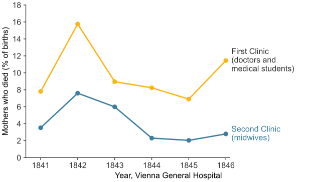
Ignaz Semmelweis, a physician in the First Clinic, later published the hospital’s annual figures for both clinics (Semmelweis 1861). Figure 22.1 shows the fraction of mothers who died in each clinic from 1841 to 1846.
Figure 22.1: Maternal deaths as a percentage of births in the two maternity clinics of the Vienna General Hospital, 1841 to 1846. Data from (Semmelweis 1861). Generated by scripts/03_statistics/01_experimental_design/gen_experimental_design.py.
In all six years, the First Clinic’s death rate was higher than the Second Clinic’s. Over the whole period, 1,989 of 20,042 mothers died in the First Clinic (9.9%), and 691 of 17,791 died in the Second Clinic (3.9%). A mother in the First Clinic was about 2.6 times as likely to die.
This is an association between the clinic and the outcome, not yet evidence about why. The obvious explanation is the staff, but the patients could also explain it: the First Clinic may have received poorer, sicker women, or women with harder labors.
ImportantKnowledge check
Before reading on, list two differences between the patients of the two clinics that could explain Figure 22.1 without the staff being responsible. What information would you need to rule them out?
NoteAnswer
Any patient characteristic that affects death risk and differs between the clinics would do: poorer, more malnourished, or older women, or longer labors. To rule these out you would need to know how women came to be admitted to each clinic.
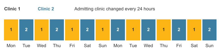
Women were not sent to a clinic according to who they were. The two clinics took turns: admission alternated every 24 hours (James Lind Library). Which clinic a woman entered depended on the day her labor started (Figure 22.2).
Figure 22.2: Admission to the two clinics alternated every 24 hours, so the clinic a woman entered depended on the day she went into labor. Generated by scripts/03_statistics/01_experimental_design/gen_experimental_design.py.
The day a woman went into labor had nothing to do with her wealth, health, or age. So women admitted to the First Clinic should, on average, resemble those admitted to the Second. The rotation made the two groups comparable. Nobody designed it as an experiment, but it produced two groups that differed mainly in one respect: who looked after them.
Physicians and medical students in the First Clinic performed autopsies, then examined women in labor. The midwives of the Second Clinic did not. Semmelweis proposed that something carried on the students’ hands from the autopsy room caused the fever. If he was right, removing it should lower the death rate.
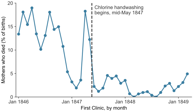
In mid-May 1847 he required the medical students to wash their hands in chlorinated lime (then called chloride of lime) before entering the First Clinic. Figure 22.3 shows the First Clinic’s monthly death rate before and after.
Figure 22.3: Maternal deaths as a percentage of births in the First Clinic, by month, January 1846 to March 1849. The dashed line marks the introduction of chlorine handwashing in mid-May 1847. Data from (Semmelweis 1861). Generated by scripts/03_statistics/01_experimental_design/gen_experimental_design.py.
In April 1847, 57 of 312 mothers died (18.3%). From June 1847 to December 1848, 101 of 5,397 died (1.9%). Over the whole of 1848 the First Clinic lost 45 of 3,556 mothers (1.3%), about the same rate as the midwives’ clinic.
Was this strong evidence that handwashing reduced deaths? Not on its own. The figure has the following limits:
The data are noisy. Monthly rates fluctuate: each month has only about 300 births. The rate had fallen to between 2% and 4% in January to March 1847, before handwashing began, then rose to 18.3% in April. A single month on either side of the line would prove nothing; the evidence is the sustained difference over many months.
Before-and-after is weaker than a side-by-side comparison. Anything else that changed in the First Clinic around May 1847 would show up as a drop in Figure 22.3.
NoteWhy this is not yet a controlled experiment
The handwashing was not assigned to patients by a random process. Semmelweis applied it to one whole clinic at once. Alternating admission made the clinics comparable, but it did not randomize the treatment.
Confounding
A causal conclusion requires accounting for other factors that might differ between the treatment and control groups.
The treatment group received the treatment. The control group did not; it shows what would have happened without the treatment.
NoteDefinition — confounding factor
A confounding factor (or confounder, or lurking variable) is any difference between the treatment and control groups, other than the treatment itself, that also affects the outcome.
A confounder can create an association even when the treatment has no effect. It can also hide a real effect, or change its size.
Example: Firefighters increase fire damage?
This example is hypothetical, with numbers chosen to make the arithmetic easy. A city compares damage from 100 fires that received many firefighters with damage from 100 fires that received few. In this city:
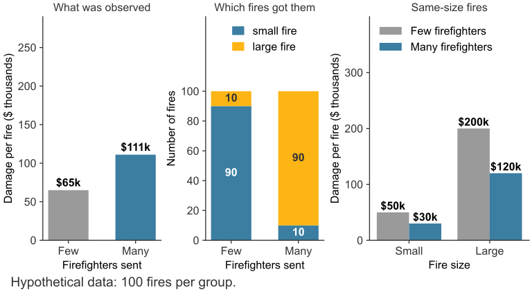
More firefighters reduce the damage. Within fires of the same size, sending many firefighters cuts the damage by 40%. A small fire that costs $50,000 with few firefighters costs $30,000 with many; a large fire that costs $200,000 costs $120,000.
Dispatchers decided how many to send, and they sent more firefighters to bigger fires. Of the 100 fires that received many firefighters, 90 were large. Of the 100 that received few, only 10 were large.
import pandas as pddamage = pd.DataFrame( # $ thousands per fire {"small": [50, 30], "large": [200, 120]}, index=["Few firefighters", "Many firefighters"],)fires = pd.DataFrame( # number of fires {"small": [90, 10], "large": [10, 90]}, index=damage.index,)fires["average damage"] = (fires["small"] * damage["small"] + fires["large"] * damage["large"]) /100fires
Fires with many firefighters averaged $111,000 of damage and fires with few averaged $65,000. Judged by that comparison alone, many firefighters appear to raise the damage by 70%. Figure 22.4 shows why this is wrong.
Figure 22.4: A hypothetical comparison of fire damage. Left: average damage as observed. Center: dispatchers sent many firefighters mostly to large fires. Right: comparing fires of the same size, many firefighters reduce the damage. Generated by scripts/03_statistics/01_experimental_design/gen_experimental_design.py.
Fire size is a confounder: it differs between the groups (center panel) and affects the outcome on its own (a large fire does about four times the damage of a small one). Comparing like with like, small fires with small and large with large (right panel), the effect reverses: many firefighters reduce the damage in both.
This pattern has a name: confounding(Kyriacou and Lewis 2016). It occurs when clinicians choose treatments because of the patient’s condition, as dispatchers chose crews because of the fire, and the condition affects the outcome.
ImportantKnowledge check
In the example above we could remove the confounding because we had recorded fire size. Suppose instead that dispatchers sent more firefighters to fires they judged “likely to spread”, and nobody recorded that judgment. Could you correct for it?
NoteAnswer
No. You can only compare like with like for factors you have measured. An unrecorded judgment, or any factor nobody thought to measure, can confound a comparison with no trace in the data. Randomization balances such factors on average, whether or not anyone measured them.
Randomization
The fire records were misleading because a person chose how many firefighters each fire received, and the choice depended on the fire. The same happens when a clinician chooses who receives treatment. Randomization takes the choice away from anyone who knows the patient.
In a randomized controlled experiment (or randomized controlled trial), each participant is assigned to the treatment or control group at random, typically by a computer’s random number generator. The treatment group then receives the treatment. Because assignment ignores the participant’s characteristics, measured and unmeasured ones are balanced between the two groups on average, by chance alone.
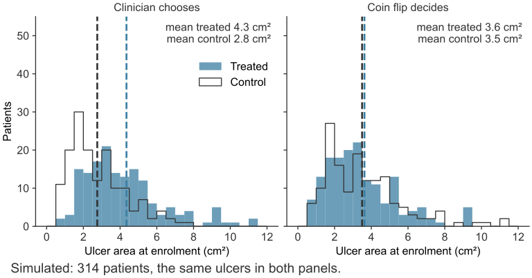
Figure 22.5 compares two ways of splitting the same 314 simulated patients, with the same ulcers, into treated and control groups: on the left by a clinician’s selection, on the right by a coin flip.
Figure 22.5: Simulated ulcer areas for 314 patients. Left: a clinician who reserves the new treatment for the larger, more worrying ulcers produces a treated group whose ulcers are larger on average. Right: a coin flip produces groups with nearly the same ulcer-size distribution. The dashed lines mark group means. Generated by scripts/03_statistics/01_experimental_design/gen_experimental_design.py.
A clinician might sensibly give the new treatment to the worst ulcers. Then the treated ulcers average 4.3 cm² and the control ulcers 2.8 cm². Because large ulcers heal slower, this would make an effective treatment look worse than it is, just as the fire records made firefighters look harmful. With randomization, the averages are 3.6 cm² and 3.5 cm². The coin flip does not make the groups identical; the histograms differ a little, and would differ more with fewer patients. Randomization guarantees only that the remaining differences are due to chance. A histogram counts the values that fall in each range. The standard deviation measures how far values typically lie from their mean.
Show the code
import numpy as nprng = np.random.default_rng(9)N =314area = rng.lognormal(mean=np.log(3.0), sigma=0.6, size=N) # cm^2, illustrative# clinician's choice: larger, more worrying ulcers are more likely to get the treatmentp_choose =1/ (1+ np.exp(-1.8* (np.log(area) - np.log(3.0))))chosen = rng.random(N) < p_choose# coin flip: every patient has probability 0.5, whatever the ulcercoin = rng.random(N) <0.5for label, treated in [("clinician chooses", chosen), ("coin flip", coin)]:print(f"{label:18s} treated mean {area[treated].mean():.1f} cm^2, "f"control mean {area[~treated].mean():.1f} cm^2")
Blinding
Randomization makes the groups alike when the study begins. The study can become biased afterward if people behave differently because they know who is in which group. A patient who knows he received a new treatment may report feeling better; a clinician who knows may assess a wound differently.
Blinding avoids this. In a blind study, participants do not know which group they are in; the control group receives a placebo, something that looks like the treatment but has no active effect. Patients often improve after a placebo; this is called the placebo effect. In a double-blind study, the people who interact with the participants or assess the outcome do not know either. Blinding is not always possible: a surgeon knows which operation she performed, and a skin substitute on a wound can be seen once applied.
In a trial of arthroscopic surgery for knee osteoarthritis, patients were randomized to lavage, debridement, or a placebo procedure without knowing which operation they received. Outcomes after either operation were no better than after the placebo (Moseley et al. 2002). The placebo allowed the trial to separate the effect of the operation from the effect of believing one had been operated on.
In a multiple sclerosis trial, two neurologists examined each patient at every visit, one blinded to the treatment and one who knew it. The blinded neurologists found no treatment superior to placebo. The unblinded neurologists’ scores showed an apparent benefit for one treatment group, a difference the blinded examinations did not support (Noseworthy et al. 1994). Both examined the same patients at the same visits, so the difference came from what each knew.
The outcome and the time at which it is measured are also fixed before the study starts. If they were chosen after the data were seen, an investigator could pick the measure that favors the treatment. With several possible outcomes or time points, one of them may favor the treatment by chance alone.
Back to Dermagraft
The Dermagraft trial was a randomized controlled trial run at 35 centers in the United States (Marston et al., 2003). Patients with diabetic foot ulcers were randomized to Dermagraft or to conventional therapy. The trial was single-blind: patients did not know which treatment they received, but the investigators did, and the efficacy analysis covers the subgroup with ulcers of more than six weeks’ duration, a subgroup identified at an interim analysis. Apart from the Dermagraft application, ulcer treatment was identical in both groups, and all patients received pressure-reducing footwear. The primary outcome was complete wound closure by week 12.
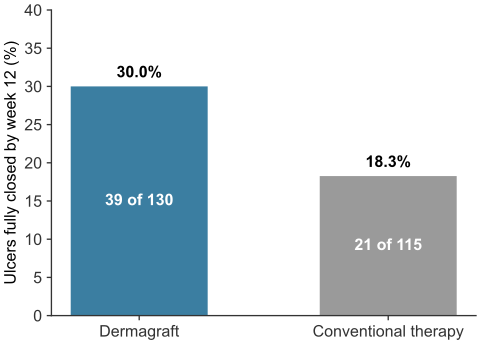
Figure 22.6: Complete wound closure by week 12 in the randomized trial of Dermagraft. Data from Marston et al. (2003). Generated by scripts/03_statistics/01_experimental_design/gen_experimental_design.py.
Of the patients analyzed, 39 of 130 in the Dermagraft group healed (30.0%), compared with 21 of 115 in the control group (18.3%) (Figure 22.6). The trial enrolled 314 patients; the healing percentages are reported for the 245 patients shown in the figure.
Because assignment was random, confounding is unlikely to explain this difference: confounders such as ulcer size, patient age, or an unmeasured factor are balanced between the groups on average. Only two explanations remain: Dermagraft improves healing, or chance assigned more of the patients who would heal anyway into the Dermagraft group. A difference of 11.7 percentage points between groups of about 120 patients could, in principle, arise by chance. The trial reported P = 0.023.
Summary
An association between a treatment and an outcome is not evidence of causation.
The most common other explanation is a confounding factor: a difference between the groups, other than the treatment, that also affects the outcome.
Comparisons are fair when the groups differ in only the treatment. Sometimes circumstances produce such groups, as alternating admission did in Vienna. Usually they must be created.
Randomization, when done correctly, creates groups that are comparable on average, except for the treatment.
Blinding keeps the treatment assignment hidden from patients and researchers, reducing bias in the assessment of outcomes.
Acknowledgement
The four-step structure (observation, a natural comparison, confounding, randomization) follows Chapter 2 of Computational and Inferential Thinking by Adhikari, DeNero and Wagner. The examples, text and figures here are original to this book.
Compute the death rate in each clinic in 1846, as a percentage of births.
How many times more likely was a mother to die in the First Clinic than in the Second Clinic in 1846?
Why did Semmelweis need the rates, rather than the raw numbers of deaths, to compare the clinics?
NoteAnswer 1
First Clinic: 459 / 4,010 = 11.4%. Second Clinic: 105 / 3,754 = 2.8%.
11.4 / 2.8 ≈ 4.1 times as likely.
The clinics delivered different numbers of babies (4,010 against 3,754 in 1846). More births means more deaths even at the same risk, so deaths must be divided by births to compare risk.
This example is hypothetical. A hospital compares infection rates between a new antimicrobial catheter coating and the standard catheter. The coating was used mostly on general wards, where patients are at lower risk of infection; the standard catheter was used mostly in intensive care.
Low-risk patients
High-risk patients
Coated catheter
150
50
Standard catheter
50
150
In this hospital, 5% of low-risk patients and 20% of high-risk patients develop an infection, whichever catheter they receive.
What percentage of patients with each catheter develop an infection?
A report concludes that the coating “roughly halves the infection rate”. Explain what is wrong with this conclusion, using the terms treatment group, control group and confounding factor.
How would you design a study to find out whether the coating reduces infection?
NoteAnswer 2
Coated: 0.05 × 150 + 0.20 × 50 = 7.5 + 10 = 17.5 infections in 200 patients, or 8.75%. Standard: 0.05 × 50 + 0.20 × 150 = 2.5 + 30 = 32.5 infections in 200 patients, or 16.25%.
The treatment group (coated catheter) and the control group (standard catheter) differ in patient risk, a confounding factor: most coated-catheter patients were low risk, and low-risk patients have fewer infections whatever catheter they receive. Within each risk level the infection rate is the same for both catheters, so the coating has no effect here. The apparent halving comes entirely from who received which catheter.
Randomize: for each eligible patient, use a chance device to decide which catheter is placed, spreading low- and high-risk patients evenly between the groups. Define the outcome (for example, a laboratory-confirmed infection within a fixed number of days) before the study begins, and have staff who do not know the patient’s catheter assess it.
Show the code
risk = {"low": 0.05, "high": 0.20}groups = {"coated": {"low": 150, "high": 50}, "standard": {"low": 50, "high": 150}}for g, n in groups.items(): infections =sum(n[k] * risk[k] for k in risk)print(f"{g:8s}{infections:.1f} of {sum(n.values())} = {100* infections /sum(n.values()):.2f}%")
TipProblem 3
You are designing a trial of a new living-skin substitute for diabetic foot ulcers, like the one in Figure 22.6.
What should the control group receive, and why is “no treatment” a poor choice?
The substitute is visible on the wound, so patients and treating clinicians will know who received it. What can you still blind, and how?
Why must the outcome, and the time at which it is measured, be fixed before the trial starts?
NoteAnswer 3
The control group should receive the best conventional care, identical in every respect except the substitute (in the Dermagraft trial, the same wound care and pressure-reducing footwear). A group given no treatment would differ from the treatment group in many ways besides the substitute, so any difference could come from the extra care rather than the substitute. Withholding standard wound care would also raise ethical problems, and would not tell a clinician whether to add the substitute to care patients already receive.
The person who judges whether the wound has closed can be blinded, for example by assessing standardized photographs of the wound without knowing the patient’s group.
If the outcome or the time point were chosen after seeing the data, an investigator could, knowingly or not, pick whichever measure made the treatment look best. With several possible outcomes and several time points, one of them may favor the treatment by chance alone.
TipProblem 4
Randomization balances the groups on average, but any single randomization leaves some chance imbalance. Using the simulated ulcer areas from the randomization section, randomize patients by coin flip and record the difference in mean ulcer area between groups. Repeat 1,000 times for trials of 20 patients and of 2,000 patients.
Plot a histogram of the 1,000 differences for each trial size.
What happens to the typical size of the chance imbalance as the trial gets bigger?
NoteAnswer 4
Show the code
import numpy as npimport matplotlib.pyplot as pltrng = np.random.default_rng(1)def imbalance(n, reps=1000): diffs = []for _ inrange(reps): area = rng.lognormal(mean=np.log(3.0), sigma=0.6, size=n) treated = rng.random(n) <0.5 diffs.append(area[treated].mean() - area[~treated].mean())return np.array(diffs)small, large = imbalance(20), imbalance(2000)bins = np.linspace(-4, 4, 41)plt.hist(small, bins, alpha=0.6, label="20 patients")plt.hist(large, bins, alpha=0.6, label="2,000 patients")plt.xlabel("Treated minus control mean ulcer area (cm²)")plt.ylabel("Number of simulated trials")plt.legend()plt.show()print(f"typical imbalance (standard deviation): 20 patients {small.std():.2f} cm², "f"2,000 patients {large.std():.2f} cm²")
Both histograms are centered on zero, so randomization is unbiased on average at any size. The spread is much narrower for 2,000 patients: the chance imbalance shrinks as the trial grows, by a factor of about 10 when the number of patients grows by a factor of 100. The same pattern appears as the standard error of a mean in sampling.
Further reading
Diez, Çetinkaya-Rundel and Barr, OpenIntro Statistics, 4th ed. A free open textbook covering the topics of this chapter (Diez et al. 2019).
Diez, David M., Mine Çetinkaya-Rundel, and Christopher D. Barr. 2019. OpenIntro Statistics. 4th ed. OpenIntro. https://www.openintro.org/book/os/.
Kyriacou, Demetrios N., and Roger J. Lewis. 2016. “Confounding by Indication in Clinical Research.”JAMA 316 (17): 1818–19. https://doi.org/10.1001/jama.2016.16435.
Moseley, J. Bruce, Kimberly O’Malley, Nancy J. Petersen, et al. 2002. “A Controlled Trial of Arthroscopic Surgery for Osteoarthritis of the Knee.”New England Journal of Medicine 347 (2): 81–88. https://doi.org/10.1056/NEJMoa013259.
Noseworthy, John H., George C. Ebers, Margaret K. Vandervoort, et al. 1994. “The Impact of Blinding on the Results of a Randomized, Placebo-Controlled Multiple Sclerosis Clinical Trial.”Neurology 44 (1): 16–20. https://doi.org/10.1212/wnl.44.1.16.
Semmelweis, Ignaz Philipp. 1861. Die Aetiologie, Der Begriff Und Die Prophylaxis Des Kindbettfiebers. C. A. Hartleben.