29 Inference on Categorical Data
In the Dermagraft trial, \(30.0\%\) of patients treated with the engineered skin substitute healed within twelve weeks, against \(18.3\%\) of those given standard care alone. That is a difference of \(11.7\) percentage points. Randomization rules out confounding but not chance. Divide any set of patients into two arms and treat them identically, and the two healing rates will rarely come out exactly equal. The question is whether the observed difference is larger than chance could produce.
Each arm reduces to a rate: the mean of a \(0/1\) outcome, with variance \(p(1-p)\) (categorical data). Such a rate, computed from a sample of size \(n\), varies from sample to sample with standard error \(\mathrm{SE} = \sqrt{p(1-p)/n}\), and for large \(n\) it is distributed normally about the true rate (sampling distribution). These pieces combine into the hypothesis test. The test assumes the device does nothing, works out how the trial’s difference would then be distributed, and reads off the normal curve how often chance alone would produce a difference this large.
import numpy as np
import matplotlib.pyplot as plt
from math import erf, sqrt, gamma, pi

# Okabe-Ito colorblind-safe palette, used consistently across this chapter's figures.
BLUE, GOLD, GREEN, PURPLE = "#0072B2", "#E69F00", "#009E73", "#CC79A7"

# The standard normal CDF, Phi(z) = P(Z <= z), from the error function:
#     Phi(z) = (1/2) [ 1 + erf(z / sqrt(2)) ].
# This is the area tool the section reads p-values from -- the same normal curve
# the sampling section built, now used to turn a z-score into a tail probability.
def Phi(z):
    return 0.5 * (1.0 + erf(z / sqrt(2.0)))

def two_sided_normal_p(z):
    "Two-tailed p-value: the standard-normal area beyond |z| in both tails."
    return 2.0 * (1.0 - Phi(abs(z)))
Estimating a proportion: the confidence interval
The device arm’s healing rate, \(\hat p = 0.300\), is a single number. It is the best available guess at the true rate \(p\) among patients like these. But it is still a guess, built from \(130\) patients rather than every patient who might ever receive the device. A different \(130\) patients would have produced a different \(\hat p\) (sampling distribution). A point estimate alone gives no sense of how far off it might be. A confidence interval does: instead of reporting the single value \(\hat p\), it reports a range of values plausible enough to contain the true \(p\).
The range is built around the point estimate, using the same standard error. \(\hat p\) is approximately normal about \(p\), with standard error \(\mathrm{SE} = \sqrt{p(1-p)/n}\) (sampling distribution; here \(\hat p\) is substituted for the unknown \(p\) inside the square root). The normal distribution’s areas then say how far \(\hat p\) typically strays from \(p\). About \(95\%\) of the normal curve lies within \(1.96\) standard deviations of its center, so a 95% confidence interval for \(p\) is
\[ \hat p \;\pm\; 1.96 \times \mathrm{SE}, \qquad \mathrm{SE} = \sqrt{\frac{\hat p (1-\hat p)}{n}}. \]
This normal model needs the success-failure condition: \(n\hat p \ge 10\) and \(n(1-\hat p) \ge 10\). The patients must also be independent of one another. For the device arm, \(130 \times 0.300 = 39\) and \(130 \times 0.700 = 91\), both at least \(10\), so the normal model applies.
More generally, at any confidence level the interval takes the form
\[ \text{point estimate} \;\pm\; z^\star \times \mathrm{SE}, \]
Here \(z^\star\) is the normal cutoff for the chosen level (\(1.65\) for \(90\%\) confidence, \(1.96\) for \(95\%\), \(2.58\) for \(99\%\)), and \(z^\star \times \mathrm{SE}\) is called the margin of error. \(z^\star\) grows with the confidence level, so the interval widens as the required confidence rises.
What “95% confidence” means
The phrase invites a probability statement about the one interval just computed, and that reading is wrong. Before the sample is drawn, \(\hat p\) is a random quantity, and so is the interval built from it. The population parameter \(p\), by contrast, is a fixed number that does not change from sample to sample. Once a particular sample of \(130\) patients has been drawn and a particular interval computed, that interval either contains \(p\) or it does not. The “\(95\%\) confidence” label describes the procedure, not this one outcome of it: if the same sampling and interval-construction procedure were repeated many times over many samples, about \(95\%\) of the resulting intervals would contain the true \(p\). A simulation of that repetition draws \(25\) hypothetical samples of \(130\) patients from a population with the device arm’s own healing rate, and builds a \(95\%\) confidence interval from each (see Figure 29.1).
p_true, n_ci = 0.300, 130
zstar_95 = 1.96

rng = np.random.default_rng(1)
p_hats = rng.binomial(n_ci, p_true, size=25) / n_ci
se_hats = np.sqrt(p_hats * (1 - p_hats) / n_ci)
los, his = p_hats - zstar_95 * se_hats, p_hats + zstar_95 * se_hats
captures = (los <= p_true) & (p_true <= his)

print(f"{captures.sum()} of 25 simulated intervals capture the true rate p = {p_true}")
24 of 25 simulated intervals capture the true rate p = 0.3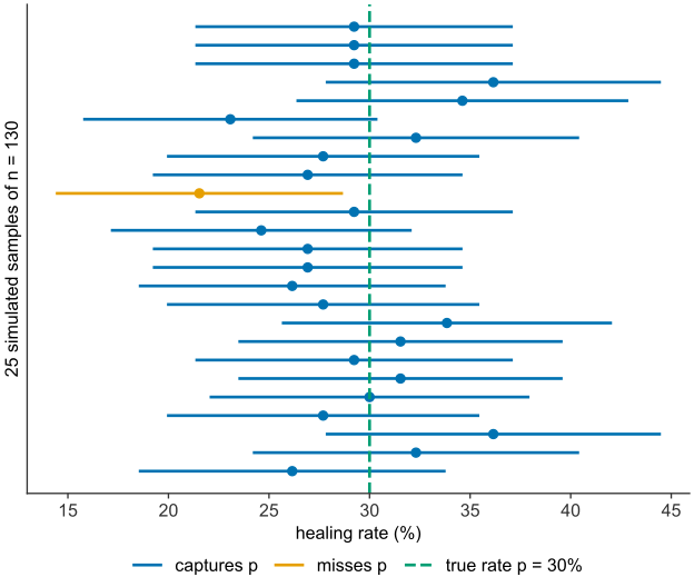
scripts/03_statistics/08_inference_categorical/gen_inference_categorical.py.
Twenty-four of the \(25\) simulated intervals contain the true rate of \(30.0\%\). One, drawn from an unusually low sample, misses it entirely.
The Dermagraft interval
The device arm’s standard error, from \(\hat p = 0.300\) on \(n = 130\) patients, is \(\mathrm{SE} \approx 4.0\) percentage points. Substituting into the \(95\%\) formula gives the interval.
p_hat, n = 0.300, 130
se = np.sqrt(p_hat * (1 - p_hat) / n)
zstar = 1.96
moe = zstar * se

print(f"p_hat = {p_hat:.3f},  SE = {se*100:.1f} percentage points")
print(f"margin of error = {moe*100:.1f} percentage points")
print(f"95% CI = ({(p_hat-moe)*100:.1f}%, {(p_hat+moe)*100:.1f}%)")
p_hat = 0.300, SE = 4.0 percentage points
margin of error = 7.9 percentage points
95% CI = (22.1%, 37.9%)The device arm’s healing rate is estimated at \(30.0\%\), and the \(95\%\) interval runs from about \(22\%\) to \(38\%\). The interval is wide, nearly \(16\) percentage points across, because it is built from only \(130\) patients. A larger trial would narrow it, since the standard error shrinks as \(1/\sqrt{n}\) (sampling distribution).
The logic of a hypothesis test
A confidence interval answers “what is the plausible range for this one rate.” The Dermagraft trial asks a comparative question: not what the device arm’s rate is on its own, but whether it differs from the control arm’s. That question needs a hypothesis test, which uses the same standard-error machinery.
A hypothesis test assumes the device does nothing, then asks how likely the observed data would be under that assumption. The assumption of no effect is the null hypothesis, written \(H_0\). The claim it is set against, that there is an effect, is the alternative hypothesis, written \(H_1\). For the trial the two read:
- \(H_0\): the device has no effect; the true healing rate is the same with it as without it, \(p_{\text{device}} = p_{\text{control}}\).
- \(H_1\): the device changes the healing rate, \(p_{\text{device}} \neq p_{\text{control}}\).
The null hypothesis is a precise, quantitative statement: it pins the two population rates to a single common value. Under \(H_0\) the sampling-distribution machinery applies approximately. If the two rates are truly equal, the observed difference \(\hat p_{\text{device}} - \hat p_{\text{control}}\) is a sample statistic with a known sampling distribution, centered on zero and spread by a standard error. This distribution, computed under \(H_0\), is the null distribution. The test locates the trial’s actual difference within it and measures how far into its tail that difference falls.
The logic is asymmetric. A test can reject the null hypothesis, meaning the data are unlikely under \(H_0\). It cannot prove \(H_0\) true. A difference consistent with chance shows only that the trial did not rule chance out, not that the device is inert. That is why a positive result is phrased as rejecting \(H_0\) rather than accepting \(H_1\).
One-sided and two-sided alternatives
The alternative hypothesis comes in two forms, and the choice between them is made before the data are seen. A two-sided (or two-tailed) alternative, \(H_1: p_{\text{device}} \neq p_{\text{control}}\), tests for a difference in either direction: the device might help or harm. It counts a result as extreme when the difference is large and positive or large and negative. A one-sided (or one-tailed) alternative, \(H_1: p_{\text{device}} > p_{\text{control}}\), tests only for a difference in a pre-specified direction, and counts only differences in that direction as evidence.
The two-sided form is the default, and the more conservative: it reserves half of the allowed error for each tail, so it demands slightly stronger evidence to reach significance in the expected direction. A one-sided test is justified only when a difference in the opposite direction would hold no interest and would be treated exactly as no difference at all. Because a device found to be worse than standard care would also be of interest, the Dermagraft comparison is two-sided.
The significance level and the p-value
Two numbers turn “how far into the tail” into a decision: a threshold fixed in advance, and the probability actually observed.
The significance level, written \(\alpha\), is the threshold: the probability of a chance result that the investigator is willing to treat as too improbable to attribute to chance. It is chosen before the data are examined, and it fixes how strong the evidence must be. By long convention \(\alpha = 0.05\): a result is declared statistically significant when it is of a kind that would arise less than five percent of the time were the null hypothesis true. The value \(0.05\) is a convention. It traces to Fisher, who in 1925 called that value “convenient” for judging significance (Fisher 1925). The p-value is the observed probability. Stated precisely:
the p-value is the probability, computed under the assumption that the null hypothesis is true, of obtaining a result at least as extreme as the one actually observed.
The p-value is computed under \(H_0\): the null is granted for argument’s sake. “At least as extreme” means a tail, not a point. The p-value adds the probability of the observed difference and of every larger one. “Extreme” is counted in the tails the alternative admits: both, for a two-sided test.
The decision rule follows mechanically. If \(p \leq \alpha\), the null is rejected; the result is statistically significant. If \(p > \alpha\), the test fails to reject \(H_0\). The same rule can be stated on the z-scale. The critical value is the cutoff that a test statistic must exceed to reject \(H_0\): for a two-sided test at \(\alpha = 0.05\), the two tails beyond \(\pm 1.96\) hold \(5\%\) of the standard normal area, so \(|z| > 1.96\) is significant.
The p-value is easy to misread. It is not the probability that \(H_0\) is true. \(H_0\) is either true or false, and the p-value is computed by assuming it true. A large p-value does not show that \(H_0\) is true; it shows only that the trial gave no evidence against it. The p-value answers one question: if the device did nothing, how often would chance alone produce a difference at least this large?
Type I and Type II error
A hypothesis test returns a verdict, and a verdict can be wrong. Because the data are random, a test can reject a true null or fail to reject a false one. There are two errors, corresponding to the two ways truth and verdict can disagree:
- A Type I error is rejecting a null hypothesis that is in fact true: declaring an effect where there is none, a false positive. Approving an inert device on the strength of a chance difference is a Type I error.
- A Type II error is failing to reject a null hypothesis that is in fact false: missing an effect that is really there, a false negative. Dismissing a device that genuinely helps, because the trial happened not to reach significance, is a Type II error.
The significance level is exactly the rate of the first error. By setting \(\alpha = 0.05\), the investigator accepts that a true null will be wrongly rejected five percent of the time: run twenty trials of treatments that do nothing, and about one will cross the threshold by chance. The probability of a Type II error is written \(\beta\). Its complement, \(1-\beta\), is the probability of correctly detecting a real effect, and it is the test’s power.
# The two error rates as areas under two competing distributions. Under H0 the
# statistic centers on 0; under a specific alternative it centers on the true effect.
# A single decision threshold (the critical value) splits both curves -- shown here
# for a one-sided test at alpha = 0.05, so the whole shaded null tail is alpha.
effect = 3.0                       # true effect size, in standard errors, under H1
zc = 1.645                         # one-sided 0.05 critical value
x = np.linspace(-4, 7, 2001)
null = np.exp(-0.5*x**2) / np.sqrt(2*pi)
alt = np.exp(-0.5*(x - effect)**2) / np.sqrt(2*pi)

fig, ax = plt.subplots(figsize=(8, 4.2))
ax.plot(x, null, color=BLUE, lw=2, label="under $H_0$ (no effect)")
ax.plot(x, alt, color=GREEN, lw=2, label="under $H_1$ (a real effect)")
ax.fill_between(x[x >= zc], null[x >= zc], color=GOLD, alpha=0.7,
                label=r"Type I error ($\alpha$): reject a true $H_0$")
ax.fill_between(x[x <= zc], alt[x <= zc], color=PURPLE, alpha=0.45,
                label=r"Type II error ($\beta$): miss a real effect")
ax.axvline(zc, color="black", lw=1.2, ls=":", label=f"decision threshold (z = {zc})")
ax.set_xlabel("test statistic")
ax.set_ylabel("density")
ax.legend(fontsize=8, loc="upper right")
plt.show()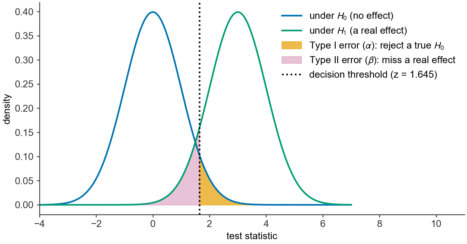
scripts/03_statistics/08_inference_categorical/gen_inference_categorical.py.
The two errors cannot both be reduced at a fixed sample size. The decision threshold is a single cutoff (see Figure 29.2). Moving it to the right, which demands a larger statistic and a smaller \(\alpha\), shrinks the Type I area and enlarges the Type II area. Moving it to the left reverses the trade. The only way to reduce both at once is to enlarge the sample. The standard error narrows as \(1/\sqrt n\) (sampling distribution), which pulls the two distributions apart.
| \(H_0\) true (no effect) | \(H_0\) false (real effect) | |
|---|---|---|
| Reject \(H_0\) (declare an effect) | Type I error (false positive, rate \(\alpha\)) | correct (power, rate \(1-\beta\)) |
| Fail to reject \(H_0\) | correct, rate \(1-\alpha\) | Type II error (false negative, rate \(\beta\)) |
The significance level \(\alpha\) is the false-positive rate the test is allowed; \(\beta\) is the false-negative rate; power \(1-\beta\) is the chance of catching a real effect.
The choice of \(\alpha\) sets how the unavoidable risk is split between false positives and false negatives. Setting \(\alpha = 0.05\) tolerates one false positive in twenty. Where a false positive is especially costly, \(\alpha\) is set lower: a definitive drug trial may demand \(0.01\) or less, and a screen that runs thousands of tests needs a far smaller threshold to keep the accumulated false positives in check. The right level depends on the relative cost of the two errors.
For the device, a Type I error would license an ineffective treatment: patients bear its cost and risk, while a wound that might have been managed otherwise goes untreated. A Type II error would shelve a device that genuinely heals, denying it to the patients it could help. The regulator requires a controlled trial, powered to detect a real benefit and judged at a pre-specified \(\alpha\), which holds both risks to a stated level.
Testing one proportion against a benchmark
The Dermagraft comparison sets two arms against each other. A single rate can also be tested against a benchmark \(p_0\). Here \(p_0 = 0.183\) is the null value, the healing rate under standard care. The device arm’s \(\hat p = 0.300\) is tested against it. The hypotheses are \(H_0: p = 0.183\) and \(H_1: p \neq 0.183\).
Under \(H_0\) the true rate is \(p_0\), so the standard error is computed from \(p_0\) rather than from \(\hat p\):
\[ \mathrm{SE}_0 = \sqrt{\frac{p_0(1-p_0)}{n}}, \qquad z = \frac{\hat p - p_0}{\mathrm{SE}_0}. \]
The normal model applies when the success-failure condition holds for \(p_0\): \(np_0 \ge 10\) and \(n(1-p_0) \ge 10\). Here \(130 \times 0.183 = 23.8\) and \(130 \times 0.817 = 106.2\), both at least \(10\).
For the device arm, \(\mathrm{SE}_0 = \sqrt{0.183 \times 0.817 / 130} = 0.0339\), so
\[ z = \frac{0.300 - 0.183}{0.0339} = 3.45, \qquad p = 2\,(1 - \Phi(3.45)) = 0.0006. \]
Since \(0.0006 < 0.05\), the null hypothesis is rejected: the device arm’s healing rate differs from the standard-care rate.
This test treats \(p_0\) as fixed, so it cannot account for variation in a second arm’s rate. The two-proportion z-test does.
When the conditions are not met
The normal model for \(\hat p\) needs independence and the success-failure condition. When the success-failure condition fails, the normal model is not accurate. A test can then use a null distribution found by simulation: draw many samples from a population with proportion \(p_0\), compute \(\hat p\) for each, and count the share at least as extreme as the observed \(\hat p\). The exact binomial probabilities from the binomial distribution give the same kind of answer for a single proportion.
When independence fails, the correction depends on how it fails. A cluster sample needs methods beyond this chapter. A convenience sample has no method that reliably corrects its bias, so its results need to be read with that bias in mind.
Choosing a sample size for a target margin of error
The confidence-interval formula runs in reverse to answer a design question asked before a trial ever enrolls a patient: how large must \(n\) be to pin down \(p\) to within a chosen margin of error \(E\)? Setting \(z^\star \mathrm{SE} \le E\) and solving for \(n\) gives
\[ n \;\ge\; \left(\frac{z^\star}{E}\right)^2 p(1-p), \]
using a planning estimate of \(p\) in place of the unknown true rate. A pilot or prior study often supplies one, such as the device arm’s own \(\hat p = 0.300\). If no estimate is available, use \(p = 0.5\). The product \(p(1-p)\) is largest at \(p = 0.5\), where it equals \(0.25\), so this choice gives the largest \(n\) for a given margin of error.
zstar, E, p_plan = 1.96, 0.05, 0.300     # target: 95% CI within +/- 5 percentage points
n_required = (zstar / E)**2 * p_plan * (1 - p_plan)
print(f"n >= {n_required:.1f}  ->  {int(np.ceil(n_required))} patients required")
n >= 322.7 -> 323 patients requiredTightening the margin of error from the trial’s actual \(\pm 7.9\) points to \(\pm 5\) points would require enrolling about \(323\) patients on the device arm alone, more than double the \(130\) actually studied.
Estimating the difference between two proportions
For two independent arms, the difference \(D = \hat p_1 - \hat p_2\) is approximately normal. Its standard error combines the two arms’ standard errors by the variances-add rule (numerical data):
\[ \mathrm{SE}_D = \sqrt{\mathrm{SE}_1^2 + \mathrm{SE}_2^2}, \qquad \mathrm{SE}_i = \sqrt{\frac{\hat p_i(1-\hat p_i)}{n_i}}. \]
The \(95\%\) confidence interval for \(p_1 - p_2\) is \(D \pm 1.96\,\mathrm{SE}_D\). Each arm’s own rate gives its standard error, since a confidence interval does not assume \(H_0\). For the Dermagraft trial, \(D = 0.300 - 0.183 = 0.117\) and \(\mathrm{SE}_D = 0.054\), so the interval is \(0.117 \pm 0.106\), or about \(1.2\) to \(22.3\) percentage points. The interval excludes zero.
Comparing two proportions: the z-test
The z-test expresses the observed difference between the two healing rates in standard errors. Under \(H_0\) both arms share one healing rate. The test therefore pools the two arms: the pooled proportion, estimated from all patients, gives the standard error of the difference and the success-failure check (sampling distribution).
The device arm healed \(39\) of \(130\) patients, giving \(\hat p_1 = 0.300\); the control arm healed \(21\) of \(115\), giving \(\hat p_2 = 0.183\). The pooled proportion is \(\hat p = 60/245 = 0.245\), so \(\mathrm{SE}_{\text{pool}} = \sqrt{0.245 \times 0.755 \times (1/130 + 1/115)} \approx 0.0551\) and \(z = 0.1174/0.0551 \approx 2.13\). The success-failure condition holds under \(H_0\) with the pooled proportion: \(0.245 \times 130 = 31.9\), \(0.755 \times 130 = 98.1\), \(0.245 \times 115 = 28.2\), and \(0.755 \times 115 = 86.8\) are all at least \(10\).
# --- The Dermagraft trial, as a two-sample z-test of two proportions ---
x1, n1 = 39, 130          # device arm:  39 of 130 healed
x2, n2 = 21, 115          # control arm: 21 of 115 healed

p1, p2 = x1 / n1, x2 / n2                 # the two observed healing rates
diff = p1 - p2                            # the observed difference

# Under H0 both arms share one rate, so the test pools them for the standard error.
p_pool = (x1 + x2) / (n1 + n2)            # pooled healing rate, from all 245 patients
se_pool = np.sqrt(p_pool * (1 - p_pool) * (1/n1 + 1/n2))

z = diff / se_pool                        # test statistic: the difference in standard errors
p_value = two_sided_normal_p(z)           # two-tailed area beyond |z|

print(f"device  rate  p1 = {p1:.3f}")
print(f"control rate  p2 = {p2:.3f}")
print(f"pooled rate   p  = {p_pool:.3f}")
print(f"observed difference  p1 - p2 = {diff*100:5.1f} percentage points")
print(f"pooled SE of the difference  = {se_pool*100:5.1f} percentage points")
print(f"z-statistic           = {z:.2f}   (the difference is {z:.2f} standard errors wide)")
print(f"two-sided p-value     = {p_value:.3f}")
device rate p1 = 0.300
control rate p2 = 0.183
pooled rate p = 0.245
observed difference p1 - p2 = 11.7 percentage points
pooled SE of the difference = 5.5 percentage points
z-statistic = 2.13 (the difference is 2.13 standard errors wide)
two-sided p-value = 0.033# Visualize the p-value as the standard-normal area beyond |z| in both tails.
grid = np.linspace(-4, 4, 2001)
density = np.exp(-0.5 * grid**2) / np.sqrt(2 * np.pi)
fig, ax = plt.subplots(figsize=(7.5, 4))
ax.plot(grid, density, color=BLUE, lw=2)
right, left = grid >= z, grid <= -z
ax.fill_between(grid[right], density[right], color=GOLD, alpha=0.6)
ax.fill_between(grid[left], density[left], color=GOLD, alpha=0.6)
ax.axvline(z, color=GREEN, lw=2, label=f"observed z = {z:.2f}")
ax.axvline(-z, color=GREEN, lw=1.2, ls="--")
ax.axvline(1.96, color="0.5", lw=1, ls=":", label="±1.96 (significance at α = 0.05)")
ax.axvline(-1.96, color="0.5", lw=1, ls=":")
ax.set_xlabel("difference in standard errors (z)")
ax.set_ylabel("standard normal density")
ax.legend(fontsize=8, loc="upper left")
plt.show()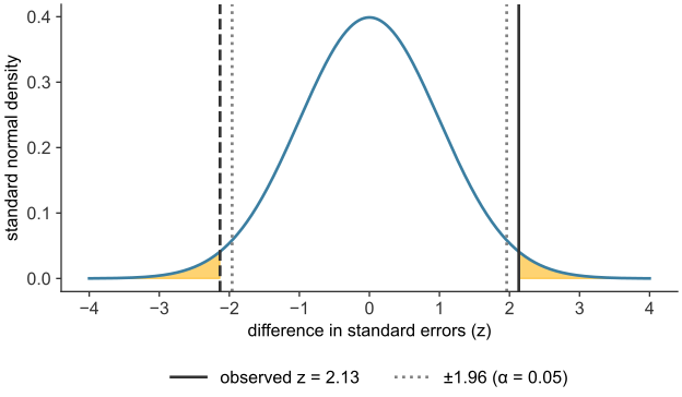
scripts/03_statistics/08_inference_categorical/gen_inference_categorical.py.
The difference between the two arms is \(z = 2.13\) standard errors wide (see Figure 29.3), and the standard normal curve places about \(3\%\) of its area that far out or farther, in the two tails combined: \(p \approx 0.033\). At the conventional threshold \(\alpha = 0.05\), the result is significant: the observed \(z\) exceeds the critical \(\pm 1.96\), so the null hypothesis of no effect is rejected. Were the device inert, a healing-rate difference as large as the trial’s would arise from chance alone about three times in a hundred.
The trial reported \(P = 0.023\) for this comparison (Marston et al. 2003). Both analyses reject the null at \(0.05\), but the values differ, and the paper explains three differences from the calculation here.
The test. The trial used a slightly different test, Fisher’s exact test, which gives the reported \(P = 0.023\) on these counts.
The population. The trial enrolled \(314\) patients. The efficacy analysis covers the \(245\) with ulcers of six weeks’ duration. The paper states that this subgroup emerged at an interim analysis, after which the analysis plan was revised to a Bayesian sequential procedure. A subgroup identified from interim data makes the reported \(P\) optimistic.
The strata. Randomization was stratified by ulcer size, \(1\) to \(2\) cm\(^2\) and \(2\) to \(20\) cm\(^2\). This test ignores those strata. The paper adjusts for ulcer area and sex only in its analysis of time to closure.
Testing counts against a model: the chi-square goodness-of-fit test
The z-test compares two rates. Many categorical questions instead compare a whole table of counts against proportions fixed by some other source, such as a model, a regulation, or a known population, and no single rate captures that comparison. Suppose a multicenter trial enrolls \(240\) patients and records each patient’s blood type, and the trial’s statisticians want to know whether the enrolled blood-type distribution matches the distribution reported for the general population. The population figures are hypothetical, rounded for illustration, and are \(45\%\) type O, \(40\%\) type A, \(11\%\) type B, and \(4\%\) type AB, using the categories from data types. If enrollment were representative, the \(240\) patients should split across the four types in roughly those proportions. If it is skewed, the trial’s result may generalize poorly to the general population.
The expected count in each category is what representative enrollment predicts: the population proportion times the sample size. At \(n = 240\), the expected counts are \(0.45 \times 240 = 108\) type O, \(96\) type A, \(26.4\) type B, and \(9.6\) type AB. The enrolled counts are \(95\) type O, \(101\) type A, \(32\) type B, and \(12\) type AB. Each observed count differs from its expected count, and the question is whether the four differences, taken together, are larger than sampling variation alone would produce.
The approximation needs each expected count should be at least \(5\), so that the discrete counts behind \(X^2\) are well approximated by the continuous chi-square curve. Here the smallest expected count is \(9.6\), which is above that floor.
from math import gamma

def chi2_pdf(x, k):
    "Chi-square density with k degrees of freedom, from the gamma function."
    x = np.asarray(x, dtype=float)
    out = np.zeros_like(x)
    pos = x > 0
    out[pos] = (x[pos] ** (k / 2 - 1) * np.exp(-x[pos] / 2)) / (2 ** (k / 2) * gamma(k / 2))
    return out

def chi2_upper_tail_p(x_obs, k):
    "Upper-tail area of the chi-square distribution beyond x_obs, by integration."
    xs = np.linspace(x_obs, x_obs + 80, 400_000)
    return np.trapezoid(chi2_pdf(xs, k), xs)

labels = ["O", "A", "B", "AB"]
national_prop = np.array([0.45, 0.40, 0.11, 0.04])
n_enrolled = 240
observed = np.array([95, 101, 32, 12], dtype=float)   # sums to 240

expected = national_prop * n_enrolled
X2 = np.sum((observed - expected) ** 2 / expected)
dof = len(labels) - 1
p_value = chi2_upper_tail_p(X2, dof)

for lab, o, e in zip(labels, observed, expected):
    print(f"{lab:>2}: observed {o:5.0f}   expected {e:6.1f}   "
          f"(O-E)^2/E = {(o - e)**2 / e:6.3f}")
print(f"\nX^2 = {X2:.3f}   df = {dof}   p-value = {p_value:.3f}")
O: observed 95 expected 108.0 (O-E)^2/E = 1.565
A: observed 101 expected 96.0 (O-E)^2/E = 0.260
B: observed 32 expected 26.4 (O-E)^2/E = 1.188
AB: observed 12 expected 9.6 (O-E)^2/E = 0.600
X^2 = 3.613 df = 3 p-value = 0.306fig, axes = plt.subplots(1, 2, figsize=(10.5, 4))
xbar = np.arange(len(labels))
width = 0.35
axes[0].bar(xbar - width/2, observed, width, color=BLUE, label="observed")
axes[0].bar(xbar + width/2, expected, width, color=GOLD, label="expected (national)")
axes[0].set_xticks(xbar); axes[0].set_xticklabels(labels)
axes[0].set_xlabel("blood type"); axes[0].set_ylabel("number of patients")
axes[0].legend(fontsize=8)
grid = np.linspace(0.001, 16, 2001)
axes[1].plot(grid, chi2_pdf(grid, dof), color=BLUE, lw=2, label=f"chi-square, df = {dof}")
tail = grid >= X2
axes[1].fill_between(grid[tail], chi2_pdf(grid[tail], dof), color=GOLD, alpha=0.6,
label=f"p-value = {p_value:.3f}")
axes[1].axvline(X2, color=GREEN, lw=2, label=f"observed $X^2$ = {X2:.2f}")
axes[1].set_xlabel("$X^2$"); axes[1].set_ylabel("density")
axes[1].legend(fontsize=8)
plt.show()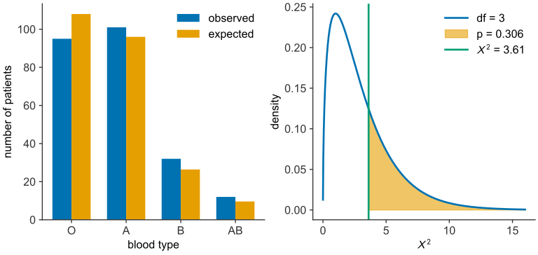
scripts/03_statistics/08_inference_categorical/gen_inference_categorical.py.
The observed counts deviate from the national proportions in each of the four categories (see Figure 29.4), but deviations of this size are within what ordinary sampling variation produces: \(X^2 = 3.61\) on three degrees of freedom gives \(p = 0.306\), far above \(0.05\). The data give no evidence that the trial’s blood-type mix differs from the national distribution. Unlike the z-test, there is no single rate to report and no single standard error. There is a table of counts and one number, \(X^2\), that summarizes how far the whole table sits from the model.
Testing association between two categorical variables: the chi-square test of independence
The goodness-of-fit test asks whether one categorical variable matches a fixed model. A second, closely related question asks whether two categorical variables, both measured on the same individuals, are related at all: whether knowing one tells you anything about the other. The z-test treats all patients in each arm as one group, across all \(35\) centers. That treatment assumes healing does not depend on center. A chi-square test of independence checks that assumption.
Consider a hypothetical three-center trial, each enrolling \(100\) patients, with healing outcomes:
| Healed | Not healed | Total | |
|---|---|---|---|
| Center A | \(40\) | \(60\) | \(100\) |
| Center B | \(55\) | \(45\) | \(100\) |
| Center C | \(45\) | \(55\) | \(100\) |
| Total | \(140\) | \(160\) | \(300\) |
If healing were independent of center, every center should show roughly the pooled rate, \(140/300 = 46.7\%\). The expected count in each cell of this two-way table comes from the table’s own row and column totals, not from an outside model:
\[ E_{\text{row},\,\text{col}} = \frac{(\text{row total}) \times (\text{column total})}{\text{table total}}. \]
For Center A’s “healed” cell, \(E = (140 \times 100)/300 = 46.7\); the same pooled rate applied to every center’s \(100\) patients. The chi-square statistic is built exactly as before, summing \((O-E)^2/E\) over every cell of the table, and its degrees of freedom for an \(r\)-row, \(c\)-column table are \((r-1)(c-1)\), here \((3-1)(2-1) = 2\).
centers = ["Center A", "Center B", "Center C"]
healed = np.array([40, 55, 45], dtype=float)
n_per_center = np.array([100, 100, 100], dtype=float)
not_healed = n_per_center - healed

table = np.vstack([healed, not_healed])                 # 2 rows (healed/not) x 3 columns (centers)
row_totals, col_totals = table.sum(axis=1), table.sum(axis=0)
expected_table = np.outer(row_totals, col_totals) / table.sum()

X2 = np.sum((table - expected_table) ** 2 / expected_table)
dof = (table.shape[0] - 1) * (table.shape[1] - 1)
p_value = chi2_upper_tail_p(X2, dof)

print("observed (healed row, not-healed row):\n", table)
print("expected:\n", np.round(expected_table, 2))
print(f"\nX^2 = {X2:.3f}   df = {dof}   p-value = {p_value:.3f}")
observed (healed row, not-healed row):
[[40. 55. 45.]
[60. 45. 55.]]
expected:
[[46.67 46.67 46.67]
[53.33 53.33 53.33]]
X^2 = 4.688 df = 2 p-value = 0.096fig, axes = plt.subplots(1, 2, figsize=(10.5, 4))
rate = healed / n_per_center
axes[0].bar(centers, rate * 100, color=BLUE)
axes[0].axhline(healed.sum() / n_per_center.sum() * 100, color=GOLD, lw=2, ls="--",
label="pooled healing rate")
axes[0].set_ylabel("healing rate (%)"); axes[0].legend(fontsize=8)
grid = np.linspace(0.001, 12, 2001)
axes[1].plot(grid, chi2_pdf(grid, dof), color=BLUE, lw=2, label=f"chi-square, df = {dof}")
tail = grid >= X2
axes[1].fill_between(grid[tail], chi2_pdf(grid[tail], dof), color=GOLD, alpha=0.6,
label=f"p-value = {p_value:.3f}")
axes[1].axvline(X2, color=GREEN, lw=2, label=f"observed $X^2$ = {X2:.2f}")
axes[1].set_xlabel("$X^2$"); axes[1].set_ylabel("density")
axes[1].legend(fontsize=8)
plt.show()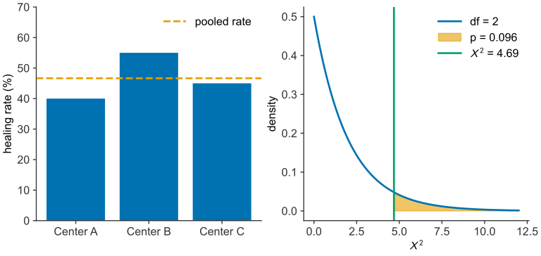
scripts/03_statistics/08_inference_categorical/gen_inference_categorical.py.
The three centers’ healing rates range from \(40\%\) to \(55\%\). The chi-square statistic, which measures this spread against chance alone, is \(X^2 = 4.69\) on two degrees of freedom, giving \(p = 0.096\) (see Figure 29.5). That is above the conventional \(\alpha = 0.05\), so the data give no evidence that healing depends on center, and pooling the centers is not contradicted. Had the p-value been small, center and outcome would not be independent, and a single pooled rate would be open to question.
When a contingency table has exactly two rows and two columns, the chi-square test of independence and the two-proportion z-test answer the same question: \(X^2\) from the chi-square test equals \(z^2\) from the (pooled) z-test on the same data. The chi-square framework is needed once a table grows past two-by-two, where no single z-statistic can summarize three or more groups at once but \(X^2\) still can.
The verdict on the device
The Dermagraft trial gave a difference in healing rates, \(30.0\%\) against \(18.3\%\). The hypothesis test asks how often chance alone would produce a difference this large if the device did nothing. The answer, about three times in a hundred, rejects that explanation at the conventional threshold: the difference is statistically significant.
That verdict rests on a chain of results: a rate is a mean, a mean has a sampling distribution, that distribution is normal with a standard error that shrinks as \(1/\sqrt n\), and a difference measured against that standard error can be graded by the normal curve into a p-value. What the p-value cannot establish is whether the trial was sound in the first place. A test grants the null its best case and weighs the data against it, but it takes the data as given: it cannot detect a trial in which the two groups differed from the start, or one in which knowing who received the device colored who was judged to have healed. Randomization and blinding make the p-value’s question valid. The chi-square test of independence lets a multicenter trial check, after the fact, whether pooling its centers was justified.
The categorical tests here cover healed or not, blood type, and center. A continuous outcome, such as how much an ulcer’s area shrank, needs its own version of this machinery (numerical inference).