35 Iodine Metabolism

The thyroid gland concentrates iodine. It draws iodide from the bloodstream through the sodium–iodide symporter, a membrane protein that co-transports the two ions into the cell. It can raise the iodide concentration inside the gland to roughly forty times the level in plasma, where the iodine is built into thyroid hormone (Pappaconstantinou et al. 2025). This avidity is the basis of a standard radiation-safety practice. A worker who handles radioactive iodine (for example Iodine-125, a common laboratory tracer) and suspects an accidental exposure can be tested: after enough time has passed for ingested iodine to move from the bloodstream into the thyroid, the gland is scanned for radioactivity (Pappaconstantinou et al. 2025). The same avidity is used in therapy: radioiodine delivered to an overactive or cancerous gland concentrates its dose in the gland (Choudhury and Gupta 2018).

How long after a suspected exposure should one wait before scanning the thyroid? Scan too early and little of the iodine has reached the gland; wait too long and the model that follows no longer applies. A model of how iodine moves from the blood into the thyroid over time answers it, using the compartmental method of the one-compartment model extended to two compartments.

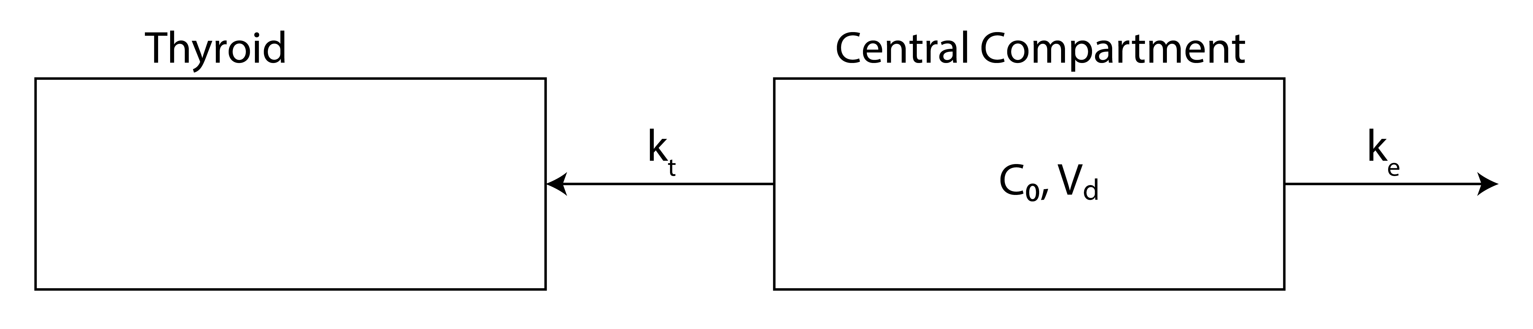
Figure 35.1: Compartmental model of ingested radioiodine. Iodine enters a central compartment (the bloodstream and the tissues it equilibrates with) and leaves it by two competing first-order routes: excretion from the body at rate constant \(k_e\) and transport into the thyroid at rate constant \(k_t\). The thyroid is a second compartment that accumulates iodine over the modeled window.

The model has two compartments (Figure 35.1). Ingested iodine passes quickly into a central compartment (the bloodstream and the well-perfused tissues it equilibrates with), from which it leaves by two competing first-order routes: excretion from the body, mostly renal (Grogan and Preuss 2023), at rate constant \(k_e\), and transport into the thyroid at rate constant \(k_t\). The thyroid is the second compartment; on the timescale of interest it accumulates iodine without releasing it. The model rests on these assumptions:

Once ingested, iodine moves quickly through the digestive system into the central compartment, so the input is effectively instantaneous.
Iodine release from the thyroid is slow compared with excretion and transport into the gland, so the return flux is neglected.
The volume of distribution of the central compartment is approximately constant.
The thyroid does not absorb so much iodine that it becomes saturated.
Before the exposure the thyroid holds no radioactive iodine.

Knowledge check

The model omits several real processes: the transit time from mouth to bloodstream, the slow release of iodine back out of the thyroid, and the physical radioactive decay of the isotope. Why is each a defensible omission for predicting the thyroid burden over the first day or two?

Answer

Each of the three processes acts on a timescale far from the one-to-two-day window the model targets. Transit from mouth to bloodstream takes minutes, short compared with the hours over which the gland fills. Release of iodine from the thyroid has a biological half-life of weeks to months (Leggett 2010), long compared with a day. Physical decay of Iodine-125 has a half-life of about 59 days, negligible over a day. Dropping a process is defensible when its timescale is far from the one being modeled.

Range of validity

The model fails at short times (minutes), because it treats movement from the mouth to the central compartment as instantaneous, and at long times (weeks), because it neglects release of iodine from the thyroid. It is built for medium times (about a day to a few days), the window relevant to deciding when to scan. The gland takes about a day to fill and empties over weeks to months, so the long-time margin is a factor of a few tens, not thousands; the model should not be used past a few days.

The central compartment

Let \(c(t)\) be the concentration of radioiodine in the central compartment and \(V_c\) its volume of distribution, the (constant) volume that converts the amount of iodine in the compartment to the measured concentration (Bisht et al. 2026). The amount of radioiodine in the compartment is then \(c\,V_c\). Iodine leaves this compartment by two first-order pathways acting in parallel: excretion from the body at rate constant \(k_e\) and transport into the thyroid at rate constant \(k_t\), each with units of inverse time. Because both removal rates are proportional to the same amount \(c\,V_c\), the mass balance for the central compartment is

\[\frac{d(c\,V_c)}{dt} = -\left(k_t + k_e\right) c\,V_c .\]

This is the single-compartment elimination equation of the one-compartment model, with the two rate constants combined into one effective removal rate \(k_t + k_e\): parallel first-order pathways add (Gibaldi and Perrier 1982). With \(V_c\) constant it divides out, leaving \(dc/dt = -(k_t+k_e)\,c\), and the concentration decays exponentially from its initial value \(c_0\),

\[c(t) = c_0\,e^{-(k_t + k_e)\,t} ,\]

with effective elimination half-life \(t_{1/2} = \ln 2/(k_t + k_e)\) (Hallare and Gerriets 2025).

The thyroid compartment

\(I(t)\) is the amount of radioiodine stored in the thyroid (for instance in millicuries), not a concentration. Iodine enters the thyroid at the transport flux \(k_t\,c\,V_c\), the same term that appears as one of the two losses in the central-compartment balance, and by assumption does not leave over the modeled window. The thyroid therefore obeys

\[\underbrace{\frac{dI}{dt}}_{\frac{\text{amount}}{\text{time}}} = \underbrace{k_t}_{\frac{1}{\text{time}}}\, \underbrace{c}_{\frac{\text{amount}}{\text{volume}}}\, \underbrace{V_c}_{\text{volume}} .\]

The units confirm the bookkeeping: a rate constant (\(1/\text{time}\)) times a concentration (\(\text{amount}/\text{volume}\)) times a volume yields an amount per unit time. The right-hand side is already known, because \(c(t)\) was found above. Substituting \(c(t) = c_0\,e^{-(k_t+k_e)t}\),

\[\frac{dI}{dt} = k_t\,V_c\,c_0\,e^{-(k_t + k_e)\,t} .\]

The right-hand side is a decaying exponential, which integrates to another exponential plus a constant,

\[I(t) = -\frac{k_t\,c_0\,V_c}{k_e + k_t}\,e^{-(k_t + k_e)\,t} + A .\]

The initial condition \(I(0) = 0\) (no radioiodine in the thyroid before the exposure) fixes the constant, \(A = k_t\,c_0\,V_c/(k_e + k_t)\). The thyroid burden is therefore

\[\boxed{\;I(t) = \frac{k_t\,c_0\,V_c}{k_e + k_t}\left(1 - e^{-(k_t + k_e)\,t}\right)\;}.\]

Since the administered dose is \(D = c_0\,V_c\), the same result reads

\[I(t) = \frac{k_t}{k_t + k_e}\,D\left(1 - e^{-(k_t + k_e)\,t}\right).\]

In this form the central volume \(V_c\) has dropped out. Predicting how much reaches the thyroid takes the amount taken in and the two rate constants, but not the volume it was spread through.

Check by substitution. \(\dfrac{dI}{dt} = \dfrac{k_t D}{k_t + k_e}\,(k_t + k_e)\,e^{-(k_t+k_e)t} = k_t D\,e^{-(k_t+k_e)t} = k_t V_c c_0\,e^{-(k_t+k_e)t}\), which matches the thyroid balance, and \(I(0) = 0\).

Key result: plateau and uptake fraction

As \(t \to \infty\) the exponential vanishes and the thyroid burden approaches a plateau,

\[ I_\infty = \frac{k_t\,c_0\,V_c}{k_e + k_t}. \]

The administered dose is \(D = c_0\,V_c\), the amount initially in the central compartment, so the fraction of the dose that ends up in the thyroid is

\[ \frac{I_\infty}{D} = \frac{k_t}{k_e + k_t}. \]

This uptake fraction is set only by the competition between the two removal pathways: the thyroid captures the share equal to its rate constant divided by the total removal rate. Faster transport into the gland (larger \(k_t\)) or slower excretion (smaller \(k_e\)) sends a larger fraction to the thyroid. The exponent \(k_t + k_e\) is the same effective rate that governs the central compartment, so the plateau is approached with time constant \(\tau = 1/(k_t + k_e)\).

The start of the curve. At \(t = 0\), \(dI/dt = k_t D\). The initial rate of uptake depends on \(k_t\) but not on \(k_e\): at the first instant, all of the iodide is still in the central compartment, and elimination has not yet taken any of it away.

The rate constants come from measured iodide kinetics in euthyroid adults (adults with normal thyroid function). Each is a clearance divided by the volume it drains, the same construction as the elimination rate constant of the one-compartment model. Absorbed iodide distributes through a volume of about 38% of body weight, mostly extracellular fluid, so \(V_c \approx 25\) L for a 65-kg adult (Rousset et al. 2015). The kidneys clear iodide from 30 to 50 mL of plasma per minute (Rousset et al. 2015; Lisco et al. 2023), with 37 mL/min as a central estimate for adult men (Leggett 2010). The thyroid clears 10 to 25 mL/min on a typical iodine intake (Rousset et al. 2015); the value falls to a few mL/min on a high iodine intake and rises above 100 mL/min in iodine deficiency (Rousset et al. 2015; Lisco et al. 2023). The thyroid’s share of the total clearance is the uptake fraction. In a euthyroid adult the measured 24-hour uptake of radioiodine typically falls between about 8% and 25% of the administered activity, and it is elevated in hyperthyroidism (Pappaconstantinou et al. 2025).

The computations below take a renal clearance of 40 mL/min and a thyroidal clearance of 10 mL/min, both inside their measured ranges, which give an uptake fraction of 20% and a total clearance of 50 mL/min. Dividing each clearance by \(V_c = 25\) L converts it to a rate constant:

\[k_e = \frac{40\ \text{mL/min} \times 60\ \text{min/h}}{25\ \text{L}} = \frac{2.4\ \text{L/h}}{25\ \text{L}} = 0.096\ \text{h}^{-1}, \qquad k_t = \frac{0.6\ \text{L/h}}{25\ \text{L}} = 0.024\ \text{h}^{-1}.\]

The sum \(k_t + k_e = 0.12\ \text{h}^{-1}\) matches the measured decline of plasma iodide of about 12% per hour (Rousset et al. 2015), and the ratio \(k_t/(k_e+k_t) = 0.20\) lies inside the euthyroid uptake range. Excretion is four times faster than transport into the gland.

Modeling the thyroid burden

Consider an initial exposure of \(2.0\) mCi of Iodine-125, distributed through a central compartment of volume \(V_c = 25\) L. The initial central concentration is then \(c_0 = (2.0\ \text{mCi})/(25\ \text{L}) = 0.08\ \text{mCi/L}\), and the administered dose is \(D = c_0\,V_c = 2.0\) mCi. With \(k_t = 0.024\ \text{h}^{-1}\) and \(k_e = 0.096\ \text{h}^{-1}\), the thyroid burden \(I(t)\) follows the boxed expression. The curve below rises from zero with time constant \(\tau = 1/(k_t+k_e) = 8.3\) h and plateaus at \(I_\infty = k_t c_0 V_c/(k_e+k_t) = 0.40\) mCi. The uptake fraction is \(k_t/(k_e+k_t) = 0.20\), so the remaining \(80\%\) of the dose is excreted. In Figure 35.2, the dashed line marks the administered dose \(D\), the upper bound on the thyroid burden. The gap between the plateau and the dose line shows that most of an administered dose never reaches the gland.

# Thyroid burden I(t): the AMOUNT of iodine in the thyroid, in the same units as the dose.
# Derived in the text:  I(t) = k_t c_0 V_c / (k_e + k_t) * (1 - exp(-(k_t + k_e) t)).
# The volume of distribution V_c converts the central concentration c into an amount;
# omitting it would return a concentration, not the thyroid amount the axis reports.
def I_t(t, k_t, k_e, c_0, V_c):
    return (k_t * c_0 * V_c) / (k_e + k_t) * (1 - np.exp(-(k_t + k_e) * t))

# Parameters (euthyroid adult; see the text for the sources)
V_c = 25.0         # iodide volume of distribution, L  (about 38% of body weight)
k_e = 0.096        # excretion rate constant, 1/hr  (renal clearance 40 mL/min / V_c)
k_t = 0.024        # transport-to-thyroid rate constant, 1/hr  (thyroid clearance 10 mL/min / V_c)
c_0 = 2.0 / 25.0   # initial central concentration, mCi/L  (2.0 mCi in 25 L)
D = c_0 * V_c      # administered dose = amount initially in central compartment, mCi

t = np.linspace(0, 40, 500)             # time, hours  (about 5 time constants of 8.3 h)
I_values = I_t(t, k_t, k_e, c_0, V_c)   # thyroid burden, mCi
I_inf = k_t * c_0 * V_c / (k_e + k_t)   # plateau (asymptote), mCi

burden_color = "#3B7EA1"   # California Blue
dose_color   = "#D55E00"   # vermilion

fig, ax = plt.subplots()
ax.plot(t, I_values, color=burden_color, lw=1.8,
        label=r'$I(t)=\dfrac{k_t c_0 V_c}{k_e+k_t}\left(1-e^{-(k_t+k_e)t}\right)$')
ax.axhline(y=D, color=dose_color, linestyle='--', lw=1.3,
           label=r'administered dose $D=c_0 V_c$ = %.1f mCi' % D)
ax.axhline(y=I_inf, color='0.6', linestyle=':', lw=1.3,
           label=r'plateau $I_\infty$ = %.2f mCi' % I_inf)
ax.set_xlabel('time (hours)')
ax.set_ylabel(r'thyroid iodine $I(t)$ (mCi)')
ax.set_ylim(0, 1.15 * D)
# legend in the clear band between the plateau and the dose line
ax.legend(loc="center right")
fig.tight_layout()
plt.show()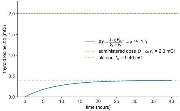

Figure 35.2: Thyroid burden \(I(t)\) for the euthyroid rate constants \(k_t = 0.024\ \text{h}^{-1}\) and \(k_e = 0.096\ \text{h}^{-1}\) (\(V_c = 25\) L), with the administered dose \(D\) (dashed) and the plateau \(I_\infty\) (dotted). The plateau is one-fifth of the dose; the gland fills with time constant \(8.3\) h.

The effect of the excretion rate \(k_e\)

Increasing the excretion rate \(k_e\) diverts a larger share of the iodine out of the body before it can reach the thyroid. The plateau \(I_\infty = k_t c_0 V_c/(k_e+k_t)\) falls, because the uptake fraction \(k_t/(k_e+k_t)\) decreases. The approach to the plateau quickens, because the time constant \(1/(k_t+k_e)\) shortens. In Figure 35.3, \(k_t = 0.024\ \text{h}^{-1}\) is held fixed while \(k_e\) varies (by the slider in the web version, from \(0.024\) to \(0.4\ \text{h}^{-1}\); the printed figure shows four values over an eightfold range). The curves leave the origin with the same slope (\(k_t D\)); curves with larger \(k_e\) then level off sooner and lower. Doubling \(k_e\) from \(0.096\) to \(0.192\ \text{h}^{-1}\) lowers the plateau from \(20\%\) to \(11\%\) of the dose and shortens \(\tau\) from \(8.3\) to \(4.6\) h. A smaller \(k_e\), as when the kidneys clear iodide more slowly, sends a larger share of the dose to the gland and takes longer to deliver it.

Knowledge check

As \(k_e\) increases, does the thyroid plateau rise or fall, and is the plateau reached sooner or later?

Answer

The plateau falls: a larger \(k_e\) lowers the uptake fraction \(k_t/(k_e+k_t)\), so less of the dose reaches the gland. It is reached sooner, because the time constant \(1/(k_t+k_e)\) shortens.

# Vary the excretion rate k_e with the transport rate k_t fixed at its euthyroid value.
# Halving k_e (for example in renal impairment) raises the uptake fraction; doubling it lowers it.
k_t = 0.024                              # 1/hr, fixed
k_e_values = [0.048, 0.096, 0.192, 0.384]
t = np.linspace(0, 72, 500)              # hours (the slowest case has a 14 h time constant)

# Berkeley palette, ordered slowest -> fastest excretion
ke_colors = ["#3B7EA1", "#FDB515", "#009E73", "#D55E00"]

fig, ax = plt.subplots()
for k_e, col in zip(k_e_values, ke_colors):
    frac = k_t / (k_t + k_e)
    ax.plot(t, I_t(t, k_t, k_e, c_0, V_c), color=col, lw=1.8,
            label=f'$k_e = {k_e}$ /hr  (uptake {100 * frac:.0f}%)')
ax.axhline(y=D, color="0.2", linestyle='--', lw=1.3,
           label=r'administered dose $D=c_0 V_c$ = %.1f mCi' % D)
ax.set_xlabel('time (hours)')
ax.set_ylabel(r'thyroid iodine $I(t)$ (mCi)')
ax.set_ylim(0, 1.15 * D)
ax.legend(loc="center right", title=r"excretion rate $k_e$ ($k_t = 0.024$ /hr)")
fig.tight_layout()
plt.show()

Figure 35.3: Thyroid burden for the chosen excretion rate constant k_e, with k_t = 0.024 per hour. The dashed grey curve is the example with k_e = 0.096 per hour.

Show the code

{
  const D = 2.0, kt = 0.024, ke = thyKe;
  const s = kt + ke, f = kt / s, tau = 1 / s;
  return html`<p><b>With k<sub>e</sub> = ${ke.toFixed(3)} h<sup>−1</sup></b> (k<sub>t</sub> = 0.024 h<sup>−1</sup>), the thyroid ends up holding <b>${(100 * f).toFixed(0)}%</b> of the dose (${(f * D).toFixed(2)} mCi of 2.0 mCi), and the gland fills with time constant τ = <b>${tau.toFixed(1)} h</b> (95% full after ${(3 * tau).toFixed(0)} h). The solid curve is this case; the dashed grey curve is the example with k<sub>e</sub> = 0.096 h<sup>−1</sup> (20% of the dose, τ = 8.3 h). Raising k<sub>e</sub> lowers the plateau and shortens τ; both curves leave the origin with the same slope, k<sub>t</sub>D.</p>`;
}

The effect of the transport rate \(k_t\)

Increasing the transport rate \(k_t\) has the opposite effect on the plateau but the same effect on the timing. A larger \(k_t\) raises the uptake fraction \(k_t/(k_e+k_t)\) toward one, so the plateau rises toward the full administered dose \(D\); it also shortens the time constant \(1/(k_t+k_e)\), so the plateau is reached sooner. In Figure 35.4, \(k_e = 0.096\ \text{h}^{-1}\) is held fixed while \(k_t\) varies (by the slider in the web version, from \(0.004\) to \(0.15\ \text{h}^{-1}\); the printed figure shows four values). With \(k_e\) at its euthyroid value, each \(k_t\) corresponds to a clinical uptake. \(k_t = 0.008\ \text{h}^{-1}\) gives an \(8\%\) uptake, the low end of the euthyroid range; \(0.024\ \text{h}^{-1}\) gives the \(20\%\) of the example; \(0.064\ \text{h}^{-1}\) gives a \(40\%\) uptake, in the hyperthyroid range; and \(0.144\ \text{h}^{-1}\) gives \(60\%\), typical of untreated Graves disease, in which the 24-hour uptake averages about \(65\%\) (Yang et al. 2023). At the other extreme, an underactive (hypothyroid) gland with \(k_t = 0.005\ \text{h}^{-1}\) takes up only \(5\%\) of the dose and fills with \(\tau = 9.9\) h. Raising \(k_t\) from the euthyroid value to \(0.144\ \text{h}^{-1}\) raises the plateau from \(20\%\) to \(60\%\) of the dose and shortens \(\tau\) from \(8.3\) to \(4.2\) h: one constant moves both answers, because \(k_t\) appears in the share and in the sum.

Knowledge check

A larger \(k_t\) and a larger \(k_e\) both make the curve reach its plateau sooner. Why, then, does raising \(k_t\) raise the plateau while raising \(k_e\) lowers it?

Answer

The time constant depends on the sum \(k_t + k_e\), so increasing either constant speeds the approach. The plateau depends on the ratio \(k_t/(k_e+k_t)\): raising \(k_t\) increases the thyroid’s share of the iodine, while raising \(k_e\) increases the competing excretion share and so decreases the thyroid’s.

# Vary the transport rate k_t with the excretion rate k_e fixed at its euthyroid value.
# The four values span the clinical range of 24-hour uptake: 8% (low end of the euthyroid
# range), 20% (euthyroid), 40% and 60% (hyperthyroid; untreated Graves disease averages about 65%).
k_e = 0.096                              # 1/hr, fixed
k_t_values = [0.008, 0.024, 0.064, 0.144]
k_t_labels = ["low-normal", "euthyroid", "hyperthyroid", "Graves disease"]
t = np.linspace(0, 48, 500)              # hours (the slowest case has a 9.6 h time constant)

# Berkeley palette, ordered slowest -> fastest transport
kt_colors = ["#3B7EA1", "#FDB515", "#009E73", "#D55E00"]

fig, ax = plt.subplots()
for k_t, name, col in zip(k_t_values, k_t_labels, kt_colors):
    frac = k_t / (k_t + k_e)
    ax.plot(t, I_t(t, k_t, k_e, c_0, V_c), color=col, lw=1.8)
    # label each curve at its right-hand end, in the clear space past the data
    ax.text(t[-1] + 1.0, I_t(t[-1], k_t, k_e, c_0, V_c),
            f'$k_t={k_t}$ /hr: {100 * frac:.0f}%, {name}', color=col, va="center", ha="left")
ax.axhline(y=D, color="0.2", linestyle='--', lw=1.3)
ax.text(1.0, D + 0.04, r'administered dose $D=c_0 V_c$ = %.1f mCi' % D, color="0.2", va="bottom")
ax.set_xlabel('time (hours)')
ax.set_ylabel(r'thyroid iodine $I(t)$ (mCi)')
ax.set_xlim(0, 84)
ax.set_ylim(0, 1.15 * D)
fig.tight_layout()
plt.show()

Figure 35.4: Thyroid burden for the chosen transport rate constant k_t, with k_e = 0.096 per hour. The dashed grey curve is the example with k_t = 0.024 per hour.

Show the code

{
  const D = 2.0, kt = thyKt, ke = 0.096;
  const s = kt + ke, f = kt / s, tau = 1 / s;
  return html`<p><b>With k<sub>t</sub> = ${kt.toFixed(3)} h<sup>−1</sup></b> (k<sub>e</sub> = 0.096 h<sup>−1</sup>), the thyroid ends up holding <b>${(100 * f).toFixed(0)}%</b> of the dose (${(f * D).toFixed(2)} mCi of 2.0 mCi), and the gland fills with time constant τ = <b>${tau.toFixed(1)} h</b> (95% full after ${(3 * tau).toFixed(0)} h). The solid curve is this case; the dashed grey curve is the example with k<sub>t</sub> = 0.024 h<sup>−1</sup> (20% of the dose, τ = 8.3 h). Raising k<sub>t</sub> raises the plateau toward the full dose and shortens τ. At 0.008 h<sup>−1</sup> the uptake is 8% (low end of normal), at 0.064 h<sup>−1</sup> it is 40% (hyperthyroid), and at 0.144 h<sup>−1</sup> it is 60% (untreated Graves disease).</p>`;
}

When to scan

The thyroid burden reaches a fraction \(1 - e^{-(k_t+k_e)t}\) of its plateau, so the time to accumulate a given fraction \(f\) is \(t = -\ln(1-f)/(k_t+k_e)\). With \(k_t + k_e = 0.12\ \text{h}^{-1}\) the gland holds \(90\%\) of its eventual burden after \(19\) hours, \(95\%\) after \(25\) hours and \(99\%\) after \(38\) hours. A scan about one day after the exposure therefore captures nearly all of the eventual thyroid burden. This agrees with clinical practice: the standard radioactive-iodine-uptake test measures the gland 24 hours after the tracer is given, sometimes with an additional early reading at 4 to 6 hours (Pappaconstantinou et al. 2025), and a detailed biokinetic model of iodine places the peak thyroid content 24 to 48 hours after intake (Leggett 2010). The 24-hour convention also standardizes the test: each laboratory’s reference range is defined at the same time point. The model’s answer and the clinical timing agree to within the spread of the measured constants: total clearance and body size move \(k_t + k_e\) over roughly \(0.10\) to \(0.15\ \text{h}^{-1}\), which moves \(t_{95}\) between about \(20\) and \(30\) hours.

The uptake fraction depends on the ratio \(k_t/(k_e+k_t)\), the time constant on the sum \(k_t + k_e\), and \(k_t\) enters both. A parameter set that overstates the fraction by making \(k_t\) too large also overstates the speed; with \(k_t\) five times \(k_e\), for instance, the model would send \(83\%\) of the dose to the gland and predict a scan within five hours. The correct fraction, \(20\%\), gives the correct timing, about a day. One day is inside the medium-time window where the model is valid: late enough that the gland has filled, early enough that neither the slow release of iodine from the thyroid nor the physical decay of Iodine-125 (half-life about 59 days) is appreciable.

The earliest detectable scan

A scanner detects the thyroid’s radioactivity only once the thyroid holds at least \(I_{\text{image}}\). The waiting time \(t_{\text{wait}}\) is when the curve crosses that level. Setting \(I(t_{\text{wait}}) = I_{\text{image}}\) and writing the plateau as \(I_\infty\),

\[I_{\text{image}} = I_\infty\left[1 - e^{-(k_t+k_e)\,t_{\text{wait}}}\right] \;\Longrightarrow\; e^{-(k_t+k_e)\,t_{\text{wait}}} = 1 - \frac{I_{\text{image}}}{I_\infty} = \frac{I_\infty - I_{\text{image}}}{I_\infty}.\]

Key result: the waiting time

\[t_{\text{wait}} = \frac{1}{k_t + k_e}\,\ln\!\left(\frac{I_\infty}{I_\infty - I_{\text{image}}}\right), \qquad I_\infty = \frac{k_t}{k_t + k_e}\,D\]

This has a solution only if \(I_{\text{image}} < I_\infty\). If the plateau is below what the scanner can detect, the logarithm is undefined: the thyroid never becomes detectable, no matter how long one waits.

Example: when can the thyroid be scanned?

Given values. The researcher takes in \(D = 2.0\) mCi of I-125, with \(k_t = 0.024\ \text{h}^{-1}\) and \(k_e = 0.096\ \text{h}^{-1}\). The thyroid is scanned at 24 h. (a) How much activity does the thyroid eventually hold, and when is it 95% full? (b) How much does it hold at the 24 h scan? (c) If the scanner can detect \(I_{\text{image}} = 0.30\) mCi, what is the earliest the scan could be done?

Time constant. \(k_t + k_e = 0.024 + 0.096 = 0.120\ \text{h}^{-1}\), so \(\tau = 1/0.120\ \text{h}^{-1} = 8.33\) h.

(a) Plateau. \(\dfrac{k_t}{k_t + k_e} = \dfrac{0.024}{0.120} = 0.20\), so \(I_\infty = 0.20 \times 2.0\ \text{mCi} = 0.40\) mCi. The other 80% leaves in the urine. The thyroid is 95% full when \(e^{-t/\tau} = 0.05\):

\[t_{95} = \tau\ln 20 = (8.33\ \text{h})(3.00) = 25.0\ \text{h}.\]

(b) At the scan. \(I(24\ \text{h}) = 0.40\ \text{mCi}\,\big(1 - e^{-(0.120)(24)}\big) = 0.40\,(1 - 0.056) = 0.38\) mCi, 94% of the plateau.

(c) Earliest detectable scan. \(I_{\text{image}} = 0.30\ \text{mCi} < I_\infty = 0.40\) mCi, so a solution exists:

\[t_{\text{wait}} = (8.33\ \text{h})\,\ln\!\left(\frac{0.40}{0.40 - 0.30}\right) = (8.33\ \text{h})\ln 4 = (8.33\ \text{h})(1.386) = 11.6\ \text{h}\]

Units. The mCi cancel inside the logarithm, and \(\tau\) carries the hours.

Result. The model is 95% full at 25 h, so the 24 h scan sees essentially the plateau. A scanner that needs only 0.30 mCi could detect the exposure after about 12 h (Figure 35.5). None of the answers needed \(V_c\).

import numpy as np

# Earliest detectable thyroid scan (given problem values; deterministic)
D, kt, ke = 2.0, 0.024, 0.096     # mCi, 1/h, 1/h
I_image   = 0.30                  # scanner threshold, mCi

s     = kt + ke
tau   = 1 / s
I_inf = kt / s * D
t95   = tau * np.log(20)
I_24  = I_inf * (1 - np.exp(-s * 24))
t_wait = tau * np.log(I_inf / (I_inf - I_image))     # needs I_image < I_inf

print(f"tau = {tau:.2f} h, I_inf = {I_inf:.2f} mCi, t95 = {t95:.1f} h")
print(f"I(24 h) = {I_24:.2f} mCi ({I_24 / I_inf:.0%} of the plateau)")
print(f"t_wait = {t_wait:.1f} h for I_image = {I_image} mCi")

tau = 8.33 h, I_inf = 0.40 mCi, t95 = 25.0 h
I(24 h) = 0.38 mCi (94% of the plateau)
t_wait = 11.6 h for I_image = 0.3 mCi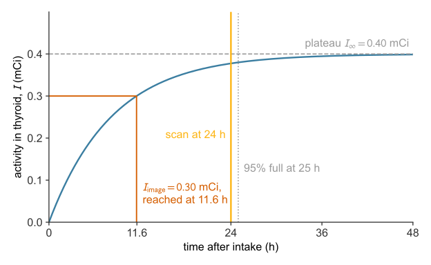

Figure 35.5: Activity in the thyroid against time for the example. The curve crosses the scanner threshold \(I_{\text{image}} = 0.30\) mCi at 11.6 h; a scan at 24 h sees 94% of the plateau of 0.40 mCi, which is 95% full at 25 h.

Optional: why radioactive decay can be ignored

I-125 decays with a half-life of 59.4 days. Decay is itself a first-order process, with rate constant

\[\lambda = \frac{\ln 2}{t_{1/2}} = \frac{0.693}{(59.4~\text{d})(24~\text{h/d})} = 4.86\times10^{-4}~\text{h}^{-1},\]

about 250 times smaller than \(k_t + k_e = 0.12\ \text{h}^{-1}\) in the example. Over 25 h, \(e^{-\lambda t} = 0.988\): decay removes about 1% of the tracer while uptake and elimination are finishing. Because decay is negligible, the activity (in mCi) stays proportional to the number of I-125 atoms, so activity can be tracked exactly as mass is. For an isotope with a short half-life this would not hold, and decay would have to be added to both mass balances as another first-order exit.

Exercises

These problems apply the two-compartment iodine model: the central-compartment decay \(c(t)=c_0 e^{-(k_t+k_e)t}\), the thyroid burden \(I(t)=\frac{k_t c_0 V_c}{k_e+k_t}\left(1-e^{-(k_t+k_e)t}\right)\), its plateau \(I_\infty\), and the uptake fraction \(k_t/(k_e+k_t)\). Unless stated otherwise, take an administered dose \(D=c_0 V_c = 2.0\) mCi (\(c_0 = 0.08\) mCi/L, \(V_c = 25\) L) and the euthyroid rate constants \(k_t = 0.024\ \text{h}^{-1}\) and \(k_e = 0.096\ \text{h}^{-1}\). Work each before revealing its answer.

Problem 1

The fraction of an administered dose that ends up in the thyroid is \(k_t/(k_e+k_t)\), and each rate constant is a clearance divided by the iodide distribution volume.

A euthyroid adult clears iodide through the kidneys at \(40\) mL/min and has \(V_c = 25\) L. Compute \(k_e\) in \(\text{h}^{-1}\).
The same adult’s measured 24-hour uptake is \(20\%\). What ratio \(k_t/k_e\) does that imply, and what is \(k_t\)?
In Graves disease the 24-hour uptake rises to about \(60\%\). If \(k_e\) is unchanged, what ratio \(k_t/k_e\) and what \(k_t\) does that imply, and by what factor has transport into the gland sped up? (Problem 5 uses the same two uptake fractions.)

Answer 1

\(k_e = (40\ \text{mL/min} \times 60\ \text{min/h})/(25\ \text{L}) = 2.4\ \text{L/h}/25\ \text{L} = \mathbf{0.096\ \text{h}^{-1}}\).
Set \(k_t/(k_e+k_t) = 0.20\). Then \(0.20(k_e+k_t) = k_t \Rightarrow 0.20\,k_e = 0.80\,k_t \Rightarrow k_t/k_e = 0.20/0.80 = \mathbf{0.25}\), so excretion is four times faster than transport into the gland and \(k_t = 0.25 \times 0.096 = \mathbf{0.024\ \text{h}^{-1}}\).
Set \(k_t/(k_e+k_t) = 0.60\): \(0.60\,k_e = 0.40\,k_t \Rightarrow k_t/k_e = \mathbf{1.5}\), so \(k_t = 1.5 \times 0.096 = \mathbf{0.144\ \text{h}^{-1}}\). Transport into the gland is \(0.144/0.024 = \mathbf{6\times}\) faster than in the euthyroid case: tripling the uptake fraction from \(0.20\) to \(0.60\) requires a sixfold rise in \(k_t\), because the fraction is a ratio bounded by one.

Problem 2

The thyroid reaches a fraction \(f = 1 - e^{-(k_t+k_e)t}\) of its plateau.

Solve for the time \(t\) to reach a fraction \(f\).
With \(k_t + k_e = 0.12\ \text{h}^{-1}\), find the times to reach \(90\%\), \(95\%\), and \(99\%\) of the plateau.
The clinical radioactive-iodine-uptake test measures the gland 24 hours after the tracer is given. Compare the model’s waiting time with this convention, and explain any discrepancy.

Answer 2

\(1 - f = e^{-(k_t+k_e)t}\), so \(t = -\dfrac{\ln(1-f)}{k_t+k_e}\).
\(t_{90} = -\ln(0.10)/0.12 = \mathbf{19\ \text{h}}\); \(t_{95} = -\ln(0.05)/0.12 = \mathbf{25\ \text{h}}\); \(t_{99} = -\ln(0.01)/0.12 = \mathbf{38\ \text{h}}\).
The model says the gland holds about \(94\%\) of its eventual burden at 24 hours (\(1 - e^{-0.12 \times 24} = 0.944\)), so the clinical timing and the model agree: one day is long enough to capture nearly all of the uptake. Doubling the wait to 48 hours recovers only \(5\%\) of the residual \(6\%\) and drifts toward the long-time regime, where release of iodine from the gland begins and the model stops applying. The clinical test fixes 24 hours rather than, say, 25 or 30 so that each laboratory’s reference range refers to the same time point; the model explains why a day is the right order of magnitude, while the exact figure is a standardization choice.

Problem 3

The central concentration decays as \(c(t) = c_0 e^{-(k_t+k_e)t}\); take \(k_t = 0.024\ \text{h}^{-1}\) and \(k_e = 0.096\ \text{h}^{-1}\).

Find the plasma (central-compartment) half-life.
What fraction of the dose remains in the central compartment at \(t = 24\) h?
At \(t = 24\) h, partition the full \(2.0\)-mCi dose among the thyroid, the excreted amount, and the central compartment, and verify the three add to the dose.

Answer 3

\(t_{1/2} = \ln 2/(k_t+k_e) = 0.693/0.12 = \mathbf{5.8\ \text{h}}\).
\(c(24)/c_0 = e^{-0.12\times 24} = e^{-2.88} = \mathbf{0.056}\), so about \(5.6\%\) remains in plasma after four half-lives.
The dose has three destinations. Central: \(0.056 \times 2.0 = 0.11\) mCi. The \(94.4\%\) that has left splits by the uptake fraction: thyroid \(0.20 \times 0.944 \times 2.0 = \mathbf{0.38\ \text{mCi}}\); excreted \(0.80 \times 0.944 \times 2.0 = 1.51\) mCi. Sum \(0.38 + 1.51 + 0.11 = \mathbf{2.0\ \text{mCi}}\), the administered dose. Mass is conserved.

Problem 4

Hold \(c_0 V_c = 2.0\) mCi.

With \(k_t = 0.024\ \text{h}^{-1}\) fixed, by what factor does \(I_\infty\) change when \(k_e\) rises from \(0.024\) to \(0.096\ \text{h}^{-1}\)?
With \(k_e = 0.096\ \text{h}^{-1}\) fixed, by what factor does \(I_\infty\) change when \(k_t\) rises from \(0.096\) to \(0.384\ \text{h}^{-1}\)?
A fourfold change was applied to each constant. Why is the effect on the plateau not fourfold in either case, and in which limit would it approach fourfold?

Answer 4

\(I_\infty = k_t c_0 V_c/(k_e+k_t) = 0.048/(k_e+0.024)\) mCi. At \(k_e = 0.024\): \(0.048/0.048 = 1.0\) mCi; at \(k_e = 0.096\): \(0.048/0.120 = 0.40\) mCi. Ratio \(\mathbf{0.40}\): the plateau falls to two-fifths.
\(I_\infty = k_t \cdot 2.0/(k_t+0.096)\). At \(k_t = 0.096\): \(0.192/0.192 = 1.0\) mCi; at \(k_t = 0.384\): \(0.768/0.480 = 1.6\) mCi. Ratio \(\mathbf{1.6}\).
The plateau depends on the ratio \(k_t/(k_e+k_t)\), which is bounded by one, not on either constant alone. In (b) the gland already captured half the dose; quadrupling \(k_t\) can at most double its share, and it reaches \(80\%\). In (a) the uptake fraction fell from \(0.50\) to \(0.20\), a factor \(2.5\) rather than \(4\), because \(k_e\) shares the denominator with \(k_t\). The response approaches fourfold only when the thyroid’s share is small (\(k_t \ll k_e\)), where the fraction is nearly \(k_t/k_e\) and scales in proportion to either constant.

Problem 5

The same avidity that makes the thyroid a sensitive exposure monitor makes radioiodine a therapy: activity delivered to the gland concentrates there.

For an administered activity of \(2.0\) mCi and a euthyroid uptake fraction of \(0.20\), how much activity settles in the thyroid at plateau?
In untreated Graves disease the 24-hour uptake fraction averages about \(0.6\) (Yang et al. 2023). How much of the same \(2.0\)-mCi activity reaches the gland, and by what factor more than the euthyroid case?
Explain, in terms of the uptake fraction, why an overactive gland receives a larger therapeutic dose at the same administered activity.

Answer 5

\(0.20 \times 2.0 = \mathbf{0.40\ \text{mCi}}\).
\(0.60 \times 2.0 = \mathbf{1.2\ \text{mCi}}\), \(\mathbf{3\times}\) the euthyroid amount.
The gland’s share of the administered activity is its uptake fraction \(k_t/(k_e+k_t)\). A hyperthyroid gland traps iodide faster (larger \(k_t\)), raising the fraction, so more of the same administered activity, and thus more radiation dose, concentrates in the target tissue while less circulates elsewhere.

Problem 6

Iodine-125 has a physical half-life of about \(59\) days; the biological accumulation has time constant \(\tau = 1/(k_t+k_e)\) with \(k_t + k_e = 0.12\ \text{h}^{-1}\).

Compute the physical decay constant \(\lambda = \ln 2/T_{1/2}\) in \(\text{h}^{-1}\).
Over the \(\sim\!25\) h needed to approach the plateau, what fraction of the Iodine-125 physically decays?
Use the two timescales to justify neglecting physical decay in the model.

Answer 6

\(T_{1/2} = 59\ \text{d} \times 24 = 1416\) h, so \(\lambda = 0.693/1416 = \mathbf{4.9\times 10^{-4}\ \text{h}^{-1}}\).
\(1 - e^{-\lambda \times 25} = 1 - e^{-1.2\times 10^{-2}} \approx \mathbf{1.2\times 10^{-2}}\), about \(1.2\%\).
The accumulation time constant (\(\tau = 1/0.12 \approx 8.3\) h) is about \(170\) times shorter than the physical half-life (\(\sim\!1400\) h), roughly two orders of magnitude. The isotope loses about one percent of its activity while it accumulates, so physical decay is negligible over the medium-time window and becomes appreciable only over the weeks the model already excludes.

Problem 7

Show that the uptake fraction can be found from the mass balance alone, without integrating the thyroid equation.

Argue that as \(t \to \infty\) all of the administered dose has left the central compartment.
The two competing pathways remove iodine from the central compartment at instantaneous rates \(k_t c V_c\) (to thyroid) and \(k_e c V_c\) (excreted). Show that the total amounts routed to each destination are in the ratio \(k_t : k_e\).
Conclude the thyroid’s share of the dose, and confirm it matches \(I_\infty/D\) from the integrated solution.

Answer 7

The central concentration decays as \(c_0 e^{-(k_t+k_e)t} \to 0\), so eventually none of the dose remains in the central compartment; by conservation of mass it has all been routed either to the thyroid or to excretion.
At any instant the two removal fluxes are \(k_t c V_c\) and \(k_e c V_c\); their ratio is \(k_t/k_e\), independent of the value of \(c(t)\). Because the ratio is the same constant at every instant, the time-integrals (the total amounts delivered to the thyroid and to excretion) are in the same ratio \(k_t : k_e\).
A dose \(D\) split in the ratio \(k_t : k_e\) sends the thyroid a fraction \(k_t/(k_t+k_e)\), so \(I_\infty = \dfrac{k_t}{k_t+k_e}\,D = \dfrac{k_t c_0 V_c}{k_e+k_t}\), identical to the plateau of the integrated solution. Competing first-order pathways split a flux in proportion to their rate constants; the explicit integration was not needed to find how the dose divides.

Problem 8

In the example, what are \(I_\infty\) and \(\tau\) if excretion doubles to \(k_e = 0.192\ \text{h}^{-1}\)? If instead uptake doubles to \(k_t = 0.048\ \text{h}^{-1}\)?

Answer 8

\(k_e = 0.192\): sum \(= 0.216\ \text{h}^{-1}\), \(\tau = 4.63\) h, \(I_\infty = (0.024/0.216)(2.0) = 0.22\) mCi. \(k_t = 0.048\): sum \(= 0.144\ \text{h}^{-1}\), \(\tau = 6.94\) h, \(I_\infty = (0.048/0.144)(2.0) = 0.67\) mCi.

Problem 9

Using the rate constants of the example and \(D = 2.0\) mCi, suppose the scanner needs \(I_{\text{image}} = 0.50\) mCi. How long must the researcher wait? What is the smallest intake the scanner could ever detect?

Answer 9

\(I_\infty = 0.40\ \text{mCi} < 0.50\) mCi, so the thyroid never becomes detectable. To be detectable at all, the plateau must exceed the threshold: \(0.20\,D > 0.50\) mCi, so the intake must exceed \(D = 2.5\) mCi. At exactly 2.5 mCi the plateau equals the threshold and is reached only as \(t \to \infty\).

Problem 10

Using the values of the example but an intake of \(D = 4.0\) mCi, find \(t_{\text{wait}}\) for \(I_{\text{image}} = 0.30\) mCi.

Answer 10

\(I_\infty = 0.20 \times 4.0 = 0.80\) mCi. \(t_{\text{wait}} = 8.33\ \text{h} \times \ln\!\big(0.80/(0.80 - 0.30)\big) = 8.33 \times \ln 1.6 = 3.9\) h. A larger intake is detectable sooner.

Problem 11

Show from the mass balance (without solving it) that the initial rate of uptake into the thyroid does not depend on \(k_e\).

Answer 11

\(dI/dt = k_t c V_c\). At \(t = 0\), \(c V_c = D\), so \(dI/dt\,|_{t=0} = k_t D\), which contains no \(k_e\). Elimination only lowers \(c\) as time goes on.

References

Bisht, Supriya, Vikas Chauhan, and Preeti Patel. 2026. “Clinical Significance of Volume of Distribution in Pharmacotherapy.” In StatPearls. StatPearls Publishing. https://www.ncbi.nlm.nih.gov/books/NBK545280/.

Choudhury, Parthajit Sengupta, and Manisha Gupta. 2018. “Differentiated Thyroid Cancer Theranostics: Radioiodine and Beyond.” The British Journal of Radiology 91: 20180136. https://doi.org/10.1259/bjr.20180136.

Gibaldi, Milo, and Donald Perrier. 1982. Pharmacokinetics. 2nd ed. Marcel Dekker.

Grogan, Sean, and Charles V. Preuss. 2023. “Pharmacokinetics.” In StatPearls. StatPearls Publishing. https://www.ncbi.nlm.nih.gov/books/NBK557744/.

Hallare, Jericho, and Valerie Gerriets. 2025. “Elimination Half-Life of Drugs.” In StatPearls. StatPearls Publishing. https://www.ncbi.nlm.nih.gov/books/NBK554498/.

Leggett, Richard W. 2010. “A Physiological Systems Model for Iodine for Use in Radiation Protection.” Radiation Research 174 (4): 496–516. https://doi.org/10.1667/RR2243.1.

Lisco, Giuseppe, Anna De Tullio, Domenico Triggiani, et al. 2023. “Iodine Deficiency and Iodine Prophylaxis: An Overview and Update.” Nutrients 15 (4): 1004. https://doi.org/10.3390/nu15041004.

Pappaconstantinou, Henry, Tyler F. Heston, and Michelle N. Tran. 2025. “I-123 Uptake.” In StatPearls. StatPearls Publishing. https://www.ncbi.nlm.nih.gov/books/NBK559314/.

Rousset, Bernard, Corinne Dupuy, Françoise Miot, and Jacques Dumont. 2015. “Thyroid Hormone Synthesis and Secretion.” In Endotext, edited by Kenneth R. Feingold, Bradley Anawalt, Marc R. Blackman, et al. MDText.com, Inc. https://www.ncbi.nlm.nih.gov/books/NBK285550/.

Yang, Qian, Wencai Ke, Fanfan Pan, Xinmei Huang, Jun Liu, and Bingbing Zha. 2023. “Association Between Radioactive Iodine Uptake and Neutropenia in Untreated Graves’ Disease.” Endocrine Connections 12 (2): e220474. https://doi.org/10.1530/EC-22-0474.