44 Capillary Flow and the Washburn Equation
A lateral flow test has no pump, yet the sample moves along the strip and reaches the test line. What pulls the sample along the strip, and how long does it take to reach the test line?
The nitrocellulose membrane of a strip is a porous medium, a tangle of connected pores (Altschuh et al. 2022). The model replaces them by straight tubes of one effective radius \(R\), with flow in each tube following Poiseuille’s law. Nothing pushes on the sample, so the driving pressure must come from the liquid surface.
Interfacial tension
Since 1 J = 1 N·m, J/m² equals N/m, so \(\gamma\) is also a force per unit length: the pull the surface exerts along a line drawn on it. For water at 20 °C, \(\gamma = 0.0728\) N/m (Urone and Hinrichs 2022).
Water molecules attract one another (cohesion), and a molecule at the surface has fewer neighbors, so creating surface costs energy (Urone and Hinrichs 2022). Attraction between unlike molecules, such as a liquid and the solid it touches, is adhesion (Urone and Hinrichs 2022).
A curved interface also carries a pressure difference, the Laplace pressure (in a capillary, the capillary pressure).
The Laplace pressure
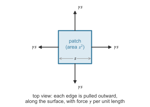
Consider a drop of fluid 2, of radius \(r_m\), in fluid 1 at equilibrium, with pressure \(P_2\) inside and \(P_1\) outside. A force balance relates the two pressures: when a body is not accelerating, the forces on it sum to zero. The body is a small square patch of the interface, of side \(s\) (Figure 44.1). The balance is written perpendicular to the patch, because the forces along the surface cancel by symmetry. Pressure pushes on the two faces of the patch, perpendicular to the surface. Surface tension pulls on each of its four edges along the surface, with force \(\gamma\) per unit length of edge.
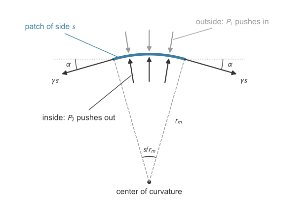
Setup. The system is the patch. Along the outward normal, \(\sum F_\perp = 0\): (force from pressure) \(-\) (inward pull of surface tension) \(= 0\).
Pressure force. The net outward push is \((P_2 - P_1)\,s^2\), the pressure difference times the patch area.
Surface-tension force. Surface tension \(\gamma\) is a force per unit length of line drawn in the surface (N/m). The surface beyond each edge of the patch pulls on the patch along the surface, perpendicular to the edge and away from the patch. An edge of length \(s\) therefore feels a pull of \(\gamma s\) (Figure 44.2). On a flat surface the pulls on opposite edges are equal and opposite, and they cancel. A curved surface leaves a net pull toward the center of curvature.
Why the pull has an inward part. The pull at an edge points along the surface at the edge, which is tilted toward the center of curvature relative to the patch’s own plane. Figure 44.3 shows a side view, with the patch centered on the top of the sphere and its right edge at \(E\).
The size of the tilt. The patch has length \(s\) along a circle of radius \(r_m\), so it spans an angle \(s/r_m\) at the center \(O\) (arc length equals radius times angle in radians). The patch is centered on the top, so its edge \(E\) lies half of that angle, \(s/(2r_m)\), away from the vertical radius to the middle of the patch. The pull at \(E\) is tangent to the sphere, so it is perpendicular to the radius \(OE\). The patch’s own plane at its middle is perpendicular to the vertical radius. The angle between two lines equals the angle between their perpendiculars, so the pull is tilted below the patch’s plane by the same angle,
\[\alpha = \frac{s}{2r_m}.\]
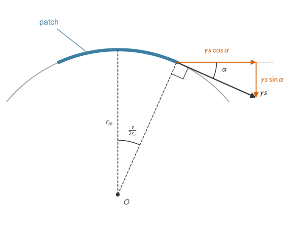
The two components. The pull \(\gamma s\) splits into a part along the patch’s plane, \(\gamma s\cos\alpha\), and a part perpendicular to it, pointing toward the center, \(\gamma s\sin\alpha\). The balance is written perpendicular to the patch, so only the inward part, \(\gamma s\sin\alpha\), enters it.
A small patch. The patch is small compared with the radius of the drop, so \(\alpha\) is small and \(\sin\alpha \approx \alpha\). For \(\alpha = 0.05\) rad, \(\sin\alpha = 0.04998\). The inward part of one edge’s pull is then
\[\gamma s\sin\alpha \approx \gamma s\cdot\frac{s}{2r_m} = \frac{\gamma s^2}{2r_m}.\]
Adding the four edges. The along-the-plane parts, \(\gamma s\cos\alpha\), of two opposite edges point in opposite directions and cancel. The two edges that point into and out of the page in the side view are tilted by the same angle, because a sphere curves equally in every direction, so each also contributes \(\gamma s^2/(2r_m)\) toward the center. The four edges together pull inward with
\[4\cdot\frac{\gamma s^2}{2r_m} = \frac{2\gamma s^2}{r_m}.\]
Balance. The outward push equals the inward pull:
\[(P_2 - P_1)\,s^2 = \frac{2\gamma s^2}{r_m} \qquad\Longrightarrow\qquad P_2 - P_1 = \frac{2\gamma}{r_m}.\]
The patch size \(s\) cancels.
A flat surface (\(r_m \to \infty\)) has no pressure jump, and a smaller drop has a higher internal pressure than a larger one. The higher pressure is on the concave side, which contains the center of curvature.
Radius of curvature in a tube
In a tube the liquid surface, the meniscus, is curved. The liquid meets the wall at the contact angle \(\theta\), measured through the liquid. The meniscus is part of a sphere (Figure 44.4, left). Let \(r_m\) be the radius of this sphere, drawn to the contact point, and \(R\) the tube radius, drawn from the axis to the wall. Because \(r_m\) is perpendicular to the meniscus and \(R\) to the wall, \(r_m\) makes the angle \(\theta\) with \(R\) (marked in the figure), so in the right triangle \(\cos\theta = R/r_m\).
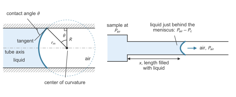
As \(\theta \to 90^\circ\), \(r_m \to \infty\): the meniscus is flat and there is no capillary pressure. At \(\theta = 0\), \(r_m = R\): the meniscus is a hemisphere and \(P_c = 2\gamma/R\) is as large as it can be.
The contact angle and the Young equation
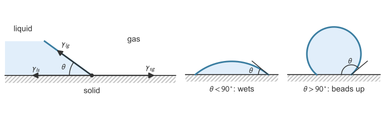
Where a liquid, a gas, and a solid meet, the solid–gas (\(\gamma_{sg}\)), liquid–solid (\(\gamma_{ls}\)), and liquid–gas (\(\gamma_{lg}\)) tensions pull on the line of contact (Figure 44.5). At equilibrium their components along the solid balance, with \(\gamma_{lg}\cos\theta\) acting in the direction of \(\gamma_{ls}\). This gives the Young equation (Gennes et al. 2004):
\[\gamma_{sg} = \gamma_{ls} + \gamma_{lg}\cos\theta \qquad\Longrightarrow\qquad \cos\theta = \frac{\gamma_{sg} - \gamma_{ls}}{\gamma_{lg}}.\]
If \(\theta < 90^\circ\), adhesion dominates and the liquid wets the surface. If \(\theta > 90^\circ\), cohesion dominates and the liquid beads up. Water on clean glass has \(\theta \approx 0^\circ\), and mercury on glass \(\theta \approx 140^\circ\) (Urone and Hinrichs 2022).
What makes the liquid front move
Consider a horizontal pore filled with liquid to length \(x\) (Figure 44.4, right). The inlet is open to the air, at \(P_\text{air}\). Just behind the meniscus the liquid is at \(P_\text{air} - P_c\), because the air is on the concave side, the side at higher pressure. The pressure falls by \(P_c\) along the liquid column, and this drop drives flow toward the meniscus, as \(\Delta P\) drives flow in a pipe.
The Washburn equation
Units: \((\text{N/m})(\text{m})(\text{s})/(\text{Pa}\cdot\text{s}) = \text{m}^2\). With the pore diameter \(D = 2R\), the equation is \(L^2 = \gamma D\cos\theta\,t/(4\mu)\). Forms without \(\cos\theta\) assume perfect wetting, \(\theta = 0\).
Because \(L\) grows as \(\sqrt{t}\), a test line twice as far away takes four times as long to reach. The front speed, \(dx/dt = \gamma R\cos\theta/(4\mu x) = x/(2t)\), falls as \(1/x\).
Where the model breaks
The pores of a real membrane are about 1 to 10 µm across (Altschuh et al. 2022). Unlike the straight, identical tubes of the model, they wind, interconnect, and vary in size. The \(R\) in the Washburn equation is therefore an effective pore radius, fitted so that the equation matches measured wicking. It absorbs these differences, so it need not equal any measured pore size (Altschuh et al. 2022). Commercial membranes are rated by their capillary flow time, the time in seconds for the liquid front to cover 4 cm of membrane (s/4 cm) (Parolo et al. 2020).
Example: wicking saliva along a test strip
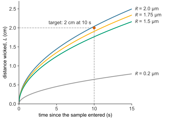
THC (tetrahydrocannabinol) is the main psychoactive compound in cannabis (Brown 2020). In a lateral flow assay for THC in saliva, the sample must reach the test line, 2 cm along the membrane, within 10 s. Assumed values for the saliva are \(\mu = 1.5\times10^{-3}\) Pa·s, a surface tension equal to water’s, rounded to \(\gamma = 0.072\) N/m, and \(\theta = 30^\circ\), so \(\cos\theta = 0.866\). The pore radii in this example, 0.2 µm and the candidates of 1.5 to 2.0 µm, are assumed effective radii, not measured pore sizes. For a membrane with \(R = 0.2\) µm, the Washburn equation gives the distance wicked in 10 s:
\[L = \sqrt{\frac{(0.072)(0.2\times10^{-6})(0.866)(10)}{2\,(1.5\times10^{-3})}} = 6.45\times10^{-3}~\text{m} = 0.645~\text{cm}.\]
This membrane wicks the saliva only 0.645 cm in 10 s, about a third of the required 2 cm. Its capillary pressure, \(P_c = 2\gamma\cos\theta/R = 6.2\times10^{5}\) Pa (about 6 atm), is large, but its narrow pores resist flow. At 10 s the front moves at \(dx/dt = L/(2t) = 0.32\) mm/s. With an assumed saliva density of 1000 kg/m³, the Reynolds number in a pore is \(\mathrm{Re} = \rho\,(dx/dt)(2R)/\mu = 8.6\times10^{-5}\), so the flow is laminar, as the model assumes. Reaching 2 cm in 10 s needs a pore radius of at least
\[R = \frac{2\mu L^2}{\gamma\cos\theta\,t} = \frac{2\,(1.5\times10^{-3})(0.02)^2}{(0.072)(0.866)(10)} = 1.92~\mu\text{m}.\]
Three membranes with assumed effective pore radii of 1.5, 1.75, and 2.0 µm are compared:
import numpy as np

mu, gamma = 1.5e-3, 0.072           # Pa s, N/m
theta = np.radians(30)              # code expects the angle in radians: 30 deg = pi/6

def wick_distance(R, t):            # Washburn: distance (m) after t (s), pore radius R (m)
    return np.sqrt(gamma * R * np.cos(theta) * t / (2 * mu))

def wick_time(R, L):                # Washburn solved for the time (s) to wick L (m)
    return 2 * mu * L**2 / (gamma * R * np.cos(theta))

for R in [1.5e-6, 1.75e-6, 2.0e-6]:
    print(f"R = {R * 1e6:.2f} um: L(10 s) = {100 * wick_distance(R, 10):.2f} cm, "
          f"time to 2 cm = {wick_time(R, 0.02):.1f} s")
R = 1.50 um: L(10 s) = 1.77 cm, time to 2 cm = 12.8 s
R = 1.75 um: L(10 s) = 1.91 cm, time to 2 cm = 11.0 s
R = 2.00 um: L(10 s) = 2.04 cm, time to 2 cm = 9.6 sOnly the 2.0 µm membrane, the one above 1.92 µm, reaches 2 cm within 10 s (Figure 44.6). Because \(L \propto \sqrt{R}\), its 33% larger pores carry the saliva only 15% farther than those of the 1.5 µm membrane.
Time to read the test
A test can be read once the sample has wicked to the test line and enough gold has bound there to be visible. The front reaches a test line a distance \(L\) away at \(t_\text{wick} = 2\mu L^2/(\gamma R\cos\theta)\): 9.6 s for a line 2 cm away on the 2.0 µm membrane of the example. The binding time \(t_\text{vis}\) (binding) is counted from the liquid’s arrival at the line, so the two times add:
\[t_\text{read} \approx t_\text{wick} + t_\text{vis} .\]
Table 44.1 applies this to the illustrative assay of binding, where \([G]_0\) is the concentration of gold-labeled antigen reaching the line.
| sample | wicking to 2 cm, \(t_\text{wick}\) | binding to visible, \(t_\text{vis}\) | total, \(t_\text{read}\) |
|---|---|---|---|
| \([G]_0 = 1\) nM | 9.6 s | 105 s | 115 s ≈ 1.9 min |
| \([G]_0 = 0.2\) nM | 9.6 s | 693 s | 703 s ≈ 11.7 min |
For these values binding, not flow, sets \(t_\text{read}\). The sum is an estimate: in a real strip, liquid keeps flowing past the test line during binding, and the binding model omits that flow. The 1 nM line is visible from 1.9 min onward, but the 0.2 nM line does not appear until 11.7 min, so the result depends on when the strip is read. Test instructions therefore fix a read time, 5 to 30 min after the sample is added (Koczula and Gallotta 2016).