41 Antibody Binding
How long does the test line take to become visible, and what is the smallest antigen concentration that can make it visible? Both answers follow from treating antibody–antigen binding as a reversible reaction and solving for the amount of complex over time.
Binding is a reversible reaction
An antibody (Ab) binds its antigen (Ag) to form a complex, Ab·Ag. The reaction runs in both directions, binding (on) and dissociation (off), each with its own rate constant:
\[\text{Ab} + \text{Ag} \;\underset{k_\text{off}}{\overset{k_\text{on}}{\rightleftharpoons}}\; \text{Ab·Ag} .\]
Square brackets denote concentration: \([\text{Ab}]\) and \([\text{Ag}]\) are the concentrations of free antibody and free antigen. The concentration of complex is written \(C\).
The rate law
Binding requires an antibody and an antigen to meet. Doubling either concentration doubles the encounter rate, so the binding rate is proportional to \([\text{Ab}][\text{Ag}]\) (the law of mass action). Dissociation needs only one complex to fall apart, so its rate is proportional to \(C\) alone:
\[\frac{dC}{dt} = \underbrace{k_\text{on}[\text{Ab}][\text{Ag}]}_{\text{complexes forming}} - \underbrace{k_\text{off}\,C}_{\text{complexes dissociating}} .\]
With concentrations in moles per liter (M), the association rate constant \(k_\text{on}\) has units of M⁻¹s⁻¹ and the dissociation rate constant \(k_\text{off}\) has units of s⁻¹, so both terms have units of M/s, matching \(dC/dt\).
The expected time course
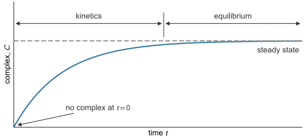
Antibody and antigen are mixed at \(t = 0\) with no complex present. Complexes form quickly at first, then more slowly as free antibody and antigen are used up and the dissociation rate rises. When the two rates balance, \(C\) stops changing: the reaction is at steady state, or equilibrium (Figure 41.1).
Equilibrium: the dissociation constant
At steady state \(dC/dt = 0\), so \(k_\text{on}[\text{Ab}][\text{Ag}] = k_\text{off}\,C\). Collecting the rate constants gives one constant for the binding pair.
\(K_D\) has units of \(\text{s}^{-1}/(\text{M}^{-1}\text{s}^{-1}) = \text{M}\), a concentration, and a smaller \(K_D\) means tighter binding, or higher affinity (Chemistry LibreTexts, n.d.). The fraction of antibody bound is \(f_b = C/([\text{Ab}] + C)\). Substituting \(C = [\text{Ab}][\text{Ag}]/K_D\),
\[f_b = \frac{[\text{Ab}][\text{Ag}]/K_D}{[\text{Ab}] + [\text{Ab}][\text{Ag}]/K_D} = \frac{[\text{Ag}]}{K_D + [\text{Ag}]} .\]
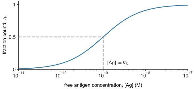
When the free antigen concentration equals \(K_D\), \(f_b = 1/2\): \(K_D\) is the antigen concentration at which half of the antibody is bound (Figure 41.2).
Exchanging antibody and antigen gives the fraction of antigen left free,
\[\frac{[\text{Ag}]}{[\text{Ag}] + C} = \frac{K_D}{K_D + [\text{Ab}]} ,\]
where \([\text{Ab}] \approx [\text{Ab}]_0\), the concentration of antibody added, when antibody far outnumbers antigen.
Each antibody–antigen pair has its own \(K_D\). Monoclonal antibodies against a single protein have measured values from single-digit picomolar to about 425 nM (Brown et al. 2020).
How long a complex lasts
The liquid flowing past the test line carries away any antigen released from its capture antibody, together with its gold label. A true positive therefore reads as negative if enough complexes dissociate before the test is read. The released antigen does not rebind, so \(k_\text{on} = 0\), the worst case. The rate law becomes \(dC/dt = -k_\text{off}C\), and from an initial value \(C_0\) at \(t = 0\) its solution is an exponential decay,
\[C = C_0\,e^{-k_\text{off} t} .\]
Setting \(C = C_0/2\) gives the half-life of the complex, \(t_{1/2} = \ln 2/k_\text{off}\), the same result as for drug elimination in the one-compartment model. A capture antibody with \(k_\text{off} = 4\times10^{-7}~\text{s}^{-1}\) (an illustrative value, not a measurement) has \(t_{1/2} = 0.693/(4\times10^{-7}~\text{s}^{-1}) = 1.73\times10^{6}\) s, about 20 days. Over a 30-minute read time, \(1 - e^{-k_\text{off}t} = 0.07\%\) of its complexes dissociate, a negligible loss.
How fast the complex forms
The starting concentrations are \([\text{Ab}]_0\), fixed when the test is made, and \([\text{Ag}]_0\), the unknown in the patient’s sample. Each complex uses one antibody and one antigen, so \([\text{Ag}] = [\text{Ag}]_0 - C\) and \([\text{Ab}] = [\text{Ab}]_0 - C\). The binding rate depends on the product of these two concentrations, and both fall as \(C\) grows. The designer supplies antibody in excess of the antigen range to be measured. If \([\text{Ab}]_0 \gg [\text{Ag}]_0\), binding every antigen uses a small fraction of the antibody, so \([\text{Ab}] \approx [\text{Ab}]_0\). With dissociation also neglected, the rate law has one variable, \(C\):
\[\frac{dC}{dt} = k_\text{on}[\text{Ab}]_0\big([\text{Ag}]_0 - C\big) .\]
Separating variables and integrating from \(C = 0\) at \(t = 0\) gives \(\ln\big([\text{Ag}]_0/([\text{Ag}]_0 - C)\big) = k_\text{on}[\text{Ab}]_0\,t\), which solves for \(t\) or \(C\):
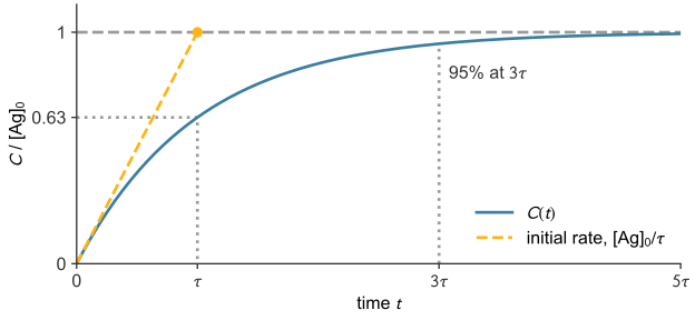
The complex closes the gap to its final value at a rate proportional to the gap. If \(C\) kept rising at its initial rate, \([\text{Ag}]_0/\tau\), it would reach the final value at \(t = \tau\) (Figure 41.3). Instead the gap shrinks by a factor of \(e\) every \(\tau\), so \(C\) is 63% complete at \(\tau\) and 95% at \(3\tau\). Setting \(C = 0.99\,[\text{Ag}]_0\) in the second form gives 99% at \(t = \tau\ln 100 \approx 4.6\,\tau\). The time constant does not depend on the antigen concentration.
The lateral flow assay as two binding reactions
In steps 2 to 4 of Figure 37.1, the sample’s antigen binds the gold-labeled detection antibody (gold–Ab) in the conjugate pad to form a complex, \(G\), which flows to the test line (step 4). There the capture antibody \(\text{Ab}_s\) binds the antigen at a second site, forming a sandwich. Colloidal gold, a suspension of gold nanoparticles, is bright red (Khlebtsov and Khlebtsov 2020), so enough sandwiches make the line visible. The two antibodies bind different sites, so the reactions have separate constants, labeled \(g\) (gold) and \(s\) (strip) (Table 41.1).
| Where | Reaction | Constants |
|---|---|---|
| conjugate pad (steps 2–3) | \(\text{Ag} + \text{gold–Ab} \rightleftharpoons G\) | \(k_{\text{on},g}\), \(k_{\text{off},g}\), \(K_{D,g}\) |
| test line (step 4) | \(G + \text{Ab}_s \rightleftharpoons \text{sandwich}\) | \(k_{\text{on},s}\), \(k_{\text{off},s}\) |
The signal comes from the second reaction:
\[\frac{dC}{dt} = k_{\text{on},s}[G][\text{Ab}_s] - k_{\text{off},s}C ,\]
with \(C\) now the sandwich concentration. The line becomes visible to the naked eye once enough gold collects in the test zone (Khlebtsov and Khlebtsov 2020). The visibility threshold \(C_\text{vis}\) is the smallest sandwich concentration the eye can see, and \(t_\text{vis}\) is the time at which \(C\) reaches \(C_\text{vis}\).
Assumptions
In the conjugate pad:
- The gold–Ab binds antigen with \(K_{D,g} \ll [\text{Ab}_g]_0\), so the unlabeled fraction \(K_{D,g}/(K_{D,g}+[\text{Ab}_g]_0)\) is near zero and the equilibrium lies far toward \(G\).
- The gold–Ab far outnumbers the antigen, so nearly every antigen is labeled and \([G]_0 = [\text{Ag}]_\text{sample}\). The free-antigen formula gives the unlabeled fraction, \(K_{D,g}/(K_{D,g} + [\text{Ab}_g]_0)\), where \([\text{Ab}_g]_0\) is the gold–Ab concentration.
At the test line:
- \(k_{\text{off},s}\,t_\text{read} \ll 1\); for \(4\times10^{-7}~\text{s}^{-1}\) over 30 minutes, 0.07% dissociates. Dissociation only removes sandwiches, so neglecting it gives the minimum time to a visible line.
- The capture antibody is in excess: few capture sites ever hold a sandwich, so \([\text{Ab}_s] \approx [\text{Ab}_s]_0\).
- The test line is a small, well-mixed volume: transport of antigen to the line and flow past it are ignored.
Mass balance at the line gives \([G] = [G]_0 - C\), where \([G]_0\) is the concentration of \(G\) arriving there.
Time to a visible line
Case A: capture antibody in excess
With assumptions 1 to 5, the test-line rate law becomes \(dC/dt = k_{\text{on},s}[\text{Ab}_s]_0([G]_0 - C)\), the equation of the key result with \([G]_0\) for \([\text{Ag}]_0\) and \([\text{Ab}_s]_0\) for \([\text{Ab}]_0\). The Case A time constant is the key result’s \(\tau = 1/(k_\text{on}[\text{Ab}]_0)\), here \(1/(k_{\text{on},s}[\text{Ab}_s]_0)\), and
\[C(t) = [G]_0\left(1 - e^{-t/\tau}\right), \qquad t_\text{vis} = \tau\,\ln\!\left(\frac{[G]_0}{[G]_0 - C_\text{vis}}\right) .\]
Case B: labeled antigen in excess
Case B rests on assumptions 1, 2, 3 and 5, with assumption 4 replaced by the condition that the labeled antigen \(G\) is in excess over the capture sites. The capture antibody is then used up, \([\text{Ab}_s] = [\text{Ab}_s]_0 - C\), while the sandwiches use a small fraction of the \(G\), so \([G] \approx [G]_0\). The rate law becomes \(dC/dt = k_{\text{on},s}[G]_0([\text{Ab}_s]_0 - C)\), with the Case B time constant \(\tau_B = 1/(k_{\text{on},s}[G]_0)\), and
\[C(t) = [\text{Ab}_s]_0\left(1 - e^{-t/\tau_B}\right), \qquad t_\text{vis} = \tau_B\,\ln\!\left(\frac{[\text{Ab}_s]_0}{[\text{Ab}_s]_0 - C_\text{vis}}\right) .\]
The capture antibody is fixed to the membrane, so in Case B the quantities \(C\), \(C_\text{vis}\) and \([\text{Ab}_s]_0\) can also be counted per area of the line, in mol/m² (Problem 7), while \([G]_0\) remains a concentration in mol/m³.
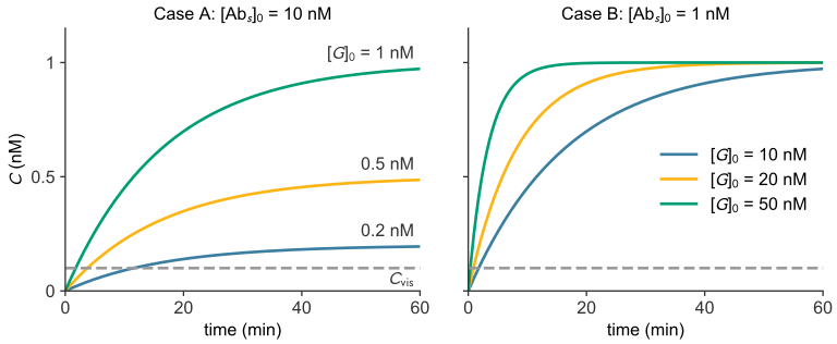
In both cases the scarce species sets the plateau and the abundant species sets the rate (Figure 41.4).
The time \(t_\text{vis}\) is counted from the moment the liquid reaches the test line. Wicking, the capillary flow of the sample along the strip (capillary flow), takes a separate time to bring the liquid there.
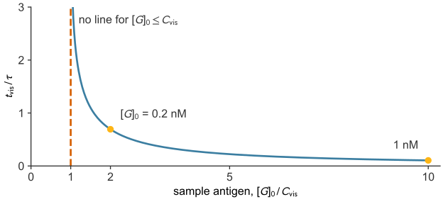
The smallest concentration that gives a line
In Case A the signal cannot exceed \([G]_0\). If \([G]_0 \le C_\text{vis}\), the logarithm is undefined, and as \([G]_0\) approaches \(C_\text{vis}\) from above, the waiting time grows without bound (Figure 41.5). Since \(C_\text{vis}\) is the smallest sandwich concentration the eye can see, no line appears in this model unless the sample’s antigen concentration exceeds \(C_\text{vis}\), however long the wait. This visibility threshold is a different criterion from the statistical limit of detection, which comes from the noise of blank readings. The LoD of diagnostic performance (in ng/mL, for the calibration assay) and \(C_\text{vis}\) (in nM, for the illustrative test here) come from different illustrative assays; a real test has one value of each in the same units, and a sample must exceed both.
In Case B the plateau is \([\text{Ab}_s]_0\), so a line can appear only if the strip is loaded with \([\text{Ab}_s]_0 > C_\text{vis}\). Then \(t_\text{vis}\) is proportional to \(\tau_B\), and so to \(1/[G]_0\). Solving the Case B result for the capture antibody gives the smallest loading that shows a line within a time \(t\) of the liquid’s arrival:
\[[\text{Ab}_s]_0 = \frac{C_\text{vis}}{1 - e^{-t/\tau_B}} .\]
The denominator is less than 1, so this loading exceeds \(C_\text{vis}\).
The hook effect
Assumption 2 holds only over the antigen range the test is designed for. A sample far above that range saturates the gold–Ab and leaves free, unlabeled antigen, which occupies capture antibodies at the test line without adding gold. Fewer colored sandwiches form, so the line gets weaker as antigen increases and can disappear, a false negative called the high-dose hook effect (Ross et al. 2020). A sandwich test therefore works from \(C_\text{vis}\) up to sample concentrations near \([\text{Ab}_g]_0\), where the gold–Ab is used up.
Example: time to a visible line
A test line has \(k_{\text{on},s} = 1\times10^{5}~\text{M}^{-1}\text{s}^{-1}\) and a capture-antibody concentration \([\text{Ab}_s]_0 = 10\) nM, and it becomes visible at \(C_\text{vis} = 0.1\) nM. How long do samples with \([G]_0 = 1\), 0.2 and 0.1 nM take? The values are illustrative, not those of a COVID-19 strip. The capture antibody is in excess (Case A), with \(\tau = 1/\big((10^{5}~\text{M}^{-1}\text{s}^{-1})(10^{-8}~\text{M})\big) = 1000\) s, and the Case A result gives each time:
import numpy as np

k_on_s, Ab_s0, C_vis = 1e5, 10e-9, 0.1e-9   # M^-1 s^-1, M, M
tau = 1 / (k_on_s * Ab_s0)

for G0 in [1e-9, 0.2e-9, 0.1e-9]:
    if G0 > C_vis:
        t_vis = tau * np.log(G0 / (G0 - C_vis))
        print(f"[G]0 = {G0 * 1e9:.1f} nM: t_vis = {t_vis:.0f} s = {t_vis / 60:.1f} min")
    else:
        print(f"[G]0 = {G0 * 1e9:.1f} nM: never visible")
[G]0 = 1.0 nM: t_vis = 105 s = 1.8 min
[G]0 = 0.2 nM: t_vis = 693 s = 11.6 min
[G]0 = 0.1 nM: never visibleA sample five times weaker takes more than six times longer, and a sample at \(C_\text{vis}\) never gives a line (Figure 41.5). Reading the test early can miss a weakly positive sample.
Back to the question
The time to read the test also includes the time the sample takes to reach the line, which follows from flow and capillary flow.