38 Calibration Curves
A strip reader scans the test line of a rapid antigen test and reports a number, for example 0.50. How much antigen was in the sample? The reader measures light, not antigen, so the number alone does not give the concentration. Converting one into the other requires a calibration curve, measured on samples of known concentration.
Analyte, sensor, and detector
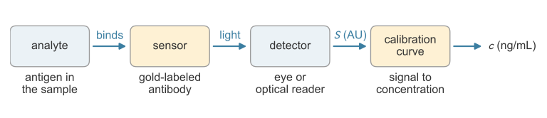
A rapid antigen test is an assay, a procedure that determines what a substance is or how much of it a sample contains. The analyte is the substance to be measured, here the antigen (Figure 38.1). A reagent is a substance added to react with the analyte. The reagent that recognizes the analyte is the sensor: in the strip, the gold-labeled detection antibody, which binds the antigen and carries a red label to the test line. The detector measures the label’s signal: the eye, or an optical reader that images the test line (Koczula and Gallotta 2016).
The detector reports a signal, not a concentration
Suppose the detector counts 10,000 photons from the test line. The count depends on the amount of analyte, and also on how much label each antibody carries, how long the detector collects light, and what fraction of that light it registers. Doubling the collection time doubles the count from the same sample. A detector’s output, written here in arbitrary units (AU), therefore has no fixed relation to concentration.
The relation is found by calibration. The assay is run on standards, samples with known concentrations of the analyte, and the calibration curve is the relation between their signals and concentrations (International Council for Harmonisation (ICH) 2022). It holds only for the reagents and detector settings it was measured with.
The calibration curve
Seven antigen standards, from a blank (0 ng/mL) to 80 ng/mL, give the signals in Table 38.1 (simulated for this illustration).
| \(c\) (ng/mL) | 0 | 5 | 10 | 20 | 40 | 60 | 80 |
|---|---|---|---|---|---|---|---|
| \(S\) (AU) | 0.050 | 0.125 | 0.170 | 0.241 | 0.547 | 0.773 | 0.984 |
The signal rises with concentration, and the points lie close to a straight line, so over this range the calibration is modeled as
\[S = a + b\,c ,\]
where the intercept \(a\) (AU) is the background signal of a sample with no analyte and the slope \(b\) (AU per ng/mL) is the signal gained per unit of concentration. If every count, background included, is proportional to the detector’s collection time, changing that time multiplies \(a\) and \(b\) by the same factor.
No line passes through all seven points. The residual of a standard is its measured signal minus the signal the line predicts (Çetinkaya-Rundel and Hardin 2024),
\[e_i = S_i - (a + b\,c_i) .\]
The least-squares line makes the sum of squared residuals, \(\text{SSE} = \sum_i e_i^2\), as small as possible (Illowsky and Dean 2023). Squaring counts every residual as positive and weights large misses most. The slope and intercept of this line are
\[b = \frac{\sum_i (c_i - \bar c)(S_i - \bar S)}{\sum_i (c_i - \bar c)^2} , \qquad a = \bar S - b\,\bar c ,\]
where \(\bar c\) and \(\bar S\) are the mean concentration and mean signal of the standards (Illowsky and Dean 2023). For Table 38.1, \(b = 0.0118\) AU per ng/mL and \(a = 0.049\) AU. The slope differs from the simulating value 0.012 by 0.0002 AU per ng/mL and the intercept from 0.040 by 0.009 AU, because of the scatter.
Judging the fit
The coefficient of determination compares the scatter left about the line with the total scatter of the signals about their mean, \(\text{SST} = \sum_i (S_i - \bar S)^2\):
\[R^2 = 1 - \frac{\text{SSE}}{\text{SST}} .\]
\(R^2\) is the fraction of the variation in the signal that the line explains, from 0 (none of it) to 1 (every point on the line) (Çetinkaya-Rundel and Hardin 2024). For Table 38.1, \(\text{SSE} = 0.0032\ \text{AU}^2\) and \(\text{SST} = 0.777\ \text{AU}^2\), so \(R^2 = 0.996\).
A high \(R^2\) does not prove that a straight line is the right model. The residuals should also scatter about zero with no pattern, as they do in Figure 38.2 (right). Residuals that are negative at both ends and positive in the middle reveal a curved response, and a straight line should not be fitted over that range (Çetinkaya-Rundel and Hardin 2024).
Reading an unknown
A sample of unknown concentration is run on the same assay, and its signal \(S^*\) is converted by solving \(S^* = a + b\,\hat c\) for the estimated concentration:
\[\hat c = \frac{S^* - a}{b} .\]
An unknown that reads \(S^* = 0.500\) AU gives \(\hat c = (0.500 - 0.049)/0.0118 = 38\) ng/mL. The slope sets how finely the assay resolves concentration. An error \(\Delta S\) in a reading becomes an error \(\Delta S/b\) in \(\hat c\), so a steeper line gives a smaller concentration error for the same signal noise. The fit, the residuals, and the reading take a few lines of code:
import numpy as np

# seven standards: known concentration c (ng/mL) and measured signal S (AU)
c = np.array([0, 5, 10, 20, 40, 60, 80])
S = np.array([0.050, 0.125, 0.170, 0.241, 0.547, 0.773, 0.984])

# least-squares slope and intercept
b = np.sum((c - c.mean()) * (S - S.mean())) / np.sum((c - c.mean())**2)
a = S.mean() - b * c.mean()

# residuals and the coefficient of determination
e = S - (a + b * c)
R2 = 1 - np.sum(e**2) / np.sum((S - S.mean())**2)

# read an unknown sample
S_star = 0.500
c_hat = (S_star - a) / b

print(f"b = {b:.4f} AU per ng/mL,  a = {a:.4f} AU,  R^2 = {R2:.3f}")
print("residuals (AU):", np.round(e, 3))
print(f"unknown: S = {S_star:.3f} AU  ->  c = {c_hat:.1f} ng/mL")
b = 0.0118 AU per ng/mL, a = 0.0493 AU, R^2 = 0.996
residuals (AU): [ 0.001 0.017 0.002 -0.045 0.024 0.013 -0.012]
unknown: S = 0.500 AU -> c = 38.1 ng/mL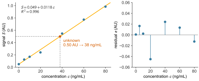
The working range
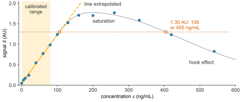
The standards of Table 38.1 span 0 to 80 ng/mL. This span, from the lowest to the highest standard, is the calibrated range (International Council for Harmonisation (ICH) 2022). Converting a signal outside it is extrapolation, which assumes the line continues where it was never measured (Çetinkaya-Rundel and Hardin 2024). The working range is the part of the calibrated range where the line still fits: its upper end is the highest standard or the point where the response stops being linear, whichever is lower, and its lower end is set by the noise of a blank.
Above about 100 ng/mL the response bends below the line and levels off (Figure 38.3) as the assay enters the capture-limited regime (Case B, defined in antibody binding), in which the capture antibody is the scarce reagent and caps the signal. An assay with capture antibody in excess (Case A, defined there) is not capped this way; its signal levels off instead when the antigen uses up the gold-labeled antibody, the onset of the hook effect described below. Binding assays calibrated up to this limit are usually fitted with a curved model instead of a line (International Council for Harmonisation (ICH) 2022). At higher concentration the signal of a sandwich test can fall. This is the high-dose hook effect (Ross et al. 2020), explained in antibody binding. On the curve of Figure 38.3, samples of 106 and 405 ng/mL then give the same signal, 1.30 AU, and the line reports both as 106 ng/mL (Table 38.2).
| Sample concentration (ng/mL) | Concentration the line reports (ng/mL) |
|---|---|
| 106 | 106 |
| 405 | 106 |
A signal above the highest standard is not extrapolated. The sample is diluted by a known factor into the calibrated range and measured again, and the result is multiplied by the dilution factor (International Council for Harmonisation (ICH) 2022). A sample far above the calibrated range can also read inside it: the 540 ng/mL standard in Figure 38.3 gives 0.83 AU, which the line reports as 66 ng/mL. Dilution does not catch this case, because the reading is already inside the range. Method validation therefore dilutes samples above the calibrated range to confirm that the hook effect does not suppress their readings (International Council for Harmonisation (ICH) 2022). At the low end, the signal approaches the background \(a\) and is lost in the scatter of blank readings, which sets the lowest detectable concentration (limit of detection).