39 Diagnostic Performance
A 2022 review pooled 152 evaluations of rapid antigen tests for COVID-19. The tests called fewer than 1% of uninfected people positive, and they detected 73.0% of infections in people with symptoms and 54.7% in people without symptoms (Dinnes et al. 2022). Why does the same strip miss more infections in one group than in another?
Laboratory studies on prepared samples measure a test’s analytical performance: how little analyte it detects, how close its readings fall to the true value and how closely they repeat, and whether it responds to other substances. A clinical study measures its clinical performance: how often its result on a patient agrees with a reference method (Saah and Hoover 1997).
Limit of detection
A blank, a sample with no analyte, still gives a signal: the 0 ng/mL standard in calibration reads 0.050 AU. Repeated blank readings scatter about a mean \(\bar S_\text{blank}\) with standard deviation \(\sigma_\text{blank}\), the spread of all the readings the blank could give. From \(n\) readings \(x_i\) with mean \(\bar x\), a standard deviation is estimated by the sample standard deviation, which divides by \(n - 1\) (numerical data):
\[s = \sqrt{\frac{1}{n-1}\sum_{i=1}^{n} (x_i - \bar x)^2} .\]
The limit of detection (LoD), also called analytical sensitivity, is the smallest amount of analyte that an assay can detect (Saah and Hoover 1997). Two other quantities are also called sensitivity: the calibration slope (Harvey 2016) and the clinical sensitivity defined below. Here, analytical sensitivity means the LoD. The statistical LoD, which sets the lower end of the working range, is the concentration whose mean signal exceeds the mean blank signal by three blank standard deviations (Harvey 2016). On the calibration line \(S = a + b\,c\), with the intercept \(a\) equal to the mean blank signal, a concentration \(c\) raises the mean signal by \(b\,c\), so the statistical LoD is
\[c_\text{LoD} = \frac{3\,\sigma_\text{blank}}{b} .\]
A smaller \(\sigma_\text{blank}\) or a steeper line lowers the LoD. A reading counts as a detection only if it exceeds the mean signal at \(c_\text{LoD}\), the threshold
\[S_\text{LoD} = \bar S_\text{blank} + 3\,\sigma_\text{blank} .\]
The factor 3 is conventional: a normally distributed blank exceeds this threshold with probability \(1 - \Phi(3) = 0.00135\), or 0.135% of the time (Harvey 2016). Here \(\Phi(z)\) is the standard normal cumulative probability, the fraction of the area under the standard normal curve that lies below \(z\) (normal distribution). The curve is symmetric, so the fraction above \(-z\) is also \(\Phi(z)\). The values needed here are \(\Phi(1) = 0.84\), \(\Phi(2) = 0.977\), and \(\Phi(3) = 0.9987\).
For the same assay (\(a = 0.049\) AU, \(b = 0.0118\) AU per ng/mL), blank strips that average 0.049 AU with a standard deviation of 0.010 AU give \(c_\text{LoD} = 0.030/0.0118 = 2.5\) ng/mL and \(S_\text{LoD} = 0.079\) AU (Figure 39.1). Low concentrations are also written in picograms per milliliter: 1 ng/mL = 1000 pg/mL, so 2.5 ng/mL = 2500 pg/mL.
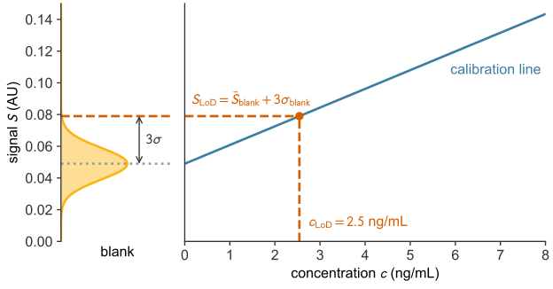
A sample at concentration \(c\) gives readings that scatter like the blank’s about the mean \(m = a + b\,c\). By the symmetry of the normal curve, a fraction \(\Phi\big((m - S_\text{LoD})/\sigma_\text{blank}\big)\) of them exceed the threshold. A sample at \(c_\text{LoD}\) has \(m = S_\text{LoD}\), so about half of its repeated tests read positive (Harvey 2016).
Under FDA guidance for COVID-19 antigen tests, the regulatory LoD is the lowest concentration detected in at least 95% of at least 20 replicates (U.S. Food and Drug Administration 2021; Blommel et al. 2023). Problem 2 tests a result by pooling a retest at that concentration with the first 20 replicates. The regulatory LoD is higher than \(c_\text{LoD}\) because it requires 95% detection, while a sample at \(c_\text{LoD}\) is detected about half the time. It needs no numeric reading, so it also applies to a strip read by eye.
Accuracy and precision
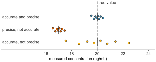
Three readers each measure a reference sample of known concentration, 20.0 ng/mL, eight times (Figure 39.2). Their readings are judged by accuracy and precision (Harvey 2016):
- Accuracy is how close the mean reading \(\bar x\) falls to the true value. It is measured by the bias, \(\bar x\) minus the true value, often given as a percentage of the true value.
- Precision is how closely the readings agree with one another. It is measured by the sample standard deviation \(s\) of the readings or by the coefficient of variation, \(\text{CV} = (s/\bar x) \times 100\%\).
Bias comes from systematic error, an error that shifts every reading the same way, as in a biased reader. Imprecision comes from random error, scatter that changes from reading to reading and averages out, so a test can have one without the other (Harvey 2016). Recalibration removes a constant bias. Averaging \(n\) readings does not remove bias, but the mean of \(n\) readings has a standard deviation of \(s/\sqrt n\) (sampling distributions). Precision within one analyst’s session is the repeatability; across analysts, days, or laboratories it is the reproducibility (Harvey 2016). The blank’s \(\sigma_\text{blank}\) is a precision at zero concentration, so a less precise reader has a higher \(c_\text{LoD}\).
Analytical specificity
An antibody can cross-react: it binds a molecule that resembles its target and produces signal with no analyte present. Other components of a real sample, such as the patient’s own antibodies or blood lipids, can interfere by adding signal or by blocking capture of the analyte. Either effect can make a result falsely high or falsely low (Tate and Ward 2004). Analytical specificity is the ability of an assay to measure its analyte and not these other substances (Saah and Hoover 1997). It is tested by adding related and interfering substances to samples and showing that they cause no false positives and do not prevent detection.
Clinical sensitivity and specificity
A clinical study tests each person with the new test and with a reference method, a laboratory test accepted as the standard of truth, usually costlier or slower. For COVID-19 antigen tests the reference is usually a test for the virus’s genetic material (Dinnes et al. 2022). Suppose 10,000 people with symptoms are tested, and the reference method finds 1,000 of them infected. Each person falls into one cell of a \(2\times2\) contingency table (Table 39.1) (Shreffler and Huecker 2023).
| Reference positive | Reference negative | Total | |
|---|---|---|---|
| Test positive | 730 true positives (TP) | 81 false positives (FP) | 811 |
| Test negative | 270 false negatives (FN) | 8919 true negatives (TN) | 9189 |
| Total | 1000 | 9000 | 10000 |
Clinical sensitivity is the fraction of infected people that the test calls positive, and clinical specificity is the fraction of uninfected people that it calls negative (Saah and Hoover 1997):
\[\begin{aligned} \text{sensitivity} &= \frac{TP}{TP + FN} = \frac{730}{1000} = 0.730 , \\[6pt] \text{specificity} &= \frac{TN}{TN + FP} = \frac{8919}{9000} = 0.991 . \end{aligned}\]
These values match the review’s summary estimates for people with symptoms (Dinnes et al. 2022). Each uses one column of the table, so neither depends on the prevalence, the fraction of the tested group that is infected (here 10%) (Shreffler and Huecker 2023). A low limit of detection does not guarantee a high clinical sensitivity (Saah and Hoover 1997), and cross-reactivity lowers clinical specificity by adding false positives (Tate and Ward 2004).
The positive predictive value (PPV) is the fraction of positive results that are correct, and the negative predictive value (NPV) is the fraction of negative results that are correct (Shreffler and Huecker 2023):
\[\begin{aligned} \text{PPV} &= \frac{TP}{TP + FP} = \frac{730}{811} = 0.900 , \\[6pt] \text{NPV} &= \frac{TN}{TN + FN} = \frac{8919}{9189} = 0.971 . \end{aligned}\]
Each uses one row, which holds both infected and uninfected people, so both depend on prevalence.
Prevalence and predictive value
Let a test have clinical sensitivity \(\text{sens}\) and clinical specificity \(\text{spec}\). In a group of \(N\) people with prevalence \(p\), it gives on average \(\text{sens}\cdot pN\) true positives and \((1-\text{spec})(1-p)N\) false positives, so
\[\text{PPV} = \frac{\text{sens}\cdot p}{\text{sens}\cdot p + (1-\text{spec})(1-p)} .\]
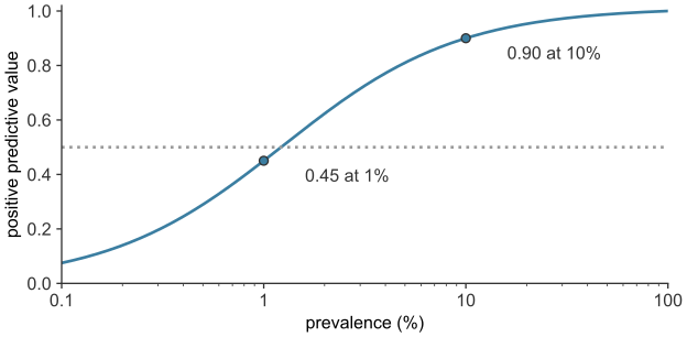
When the infection is rare, the few false positives from the large uninfected group can outnumber the true positives. The strip above has a PPV of 0.90 at 10% prevalence but 0.45 at 1%, where more than half of positive results are false (Figure 39.3).
Infected people below the limit of detection
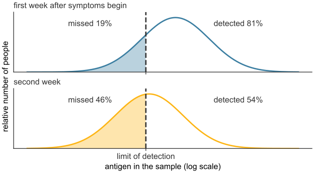
Each infected person carries a different amount of antigen. If the LoD is treated as a sharp cutoff, the strip reads positive whenever the antigen exceeds it. The clinical sensitivity is then the fraction of infected people above the LoD, and every infected person below it is a false negative (Figure 39.4). In the review, clinical sensitivity fell from 80.9% in the first week after symptoms began to 53.8% in the second. It also fell with the amount of virus in the sample, from about 98% for the samples with the most virus to under 10% for those with the least (Dinnes et al. 2022). For people without symptoms, the review suggests that part of their lower clinical sensitivity comes from timing: the period of high viral load may be shorter (Dinnes et al. 2022); a shorter window puts more of them below the LoD at testing.